Patterns of Gay Male and Lesbian Partnering in the Metropolitan Areas of the United States in 2010
 Dudley L. Poston Jr.*
 Yu-Ting Chang
- Texas A&M University, College Station, TX, USA
In this paper, we examine the degree of prevalence of partnered gay male households and partnered lesbian households in the metropolitan areas of the U.S. in 2010. We first discuss the same-sex partnering data from the 2010 U.S. Census, their biases and problems, and the adjustments researchers have developed to address the problems. We add a statistical adjustment to the data and then calculate for each of the 366 metropolitan areas of the U.S. prevalence ratios for gay male couples and for lesbian couples, and for comparative purposes, for opposite-sex cohabiting couples and opposite-sex married couples. Then, we propose and test several ecological hypotheses to account for the variability among the metropolitan areas in the partnering ratios.
Introduction
In this paper, we examine the degree of prevalence of partnered gay male households and partnered lesbian households in the metropolitan areas of the U.S. in 2010. Partnered gay males and lesbians live virtually everywhere in the U.S.; they live in all the states and metropolitan areas and in most of the counties. However, most (around 85%) live in metropolitan statistical areas (Simmons and O’Connell, 2003, p. 2; Gates and Ost, 2004; Walther et al., 2011). Also, prior research (Black et al., 2000, 2002; Gates and Ost, 2004; Walther and Poston, 2004; Walther et al., 2011; Gates, 2013; among others) shows considerable variation among the metropolitan areas with respect to the prevalence of gay male and lesbian partnering. These very different distributions of gay males and lesbians are of interest if only for the fact that they are sometimes associated with the political and social visibility of gay males and lesbians. Metropolitan areas where gay males and lesbians have settled have become, according to O’Reilly and Webster (1998), “gay spaces” with political force and activism. Metropolitan areas with the largest proportional representations of gay males and lesbians, for instance, San Francisco, New York City, Houston, and Los Angeles are among the “gay spaces” that receive the most national attention. But as just noted, there are concentrations of gay males and lesbians in virtually all the metropolitan areas of the country, and these patterns and distributions are sometimes overlooked in research on gay males and lesbians.
There are several analyses of gay male and lesbian partner prevalence patterns using 1990 and 2000 U.S. census data (for examples, see Black et al., 2000, 2002; Gates and Ost, 2004; Walther and Poston, 2004; Baumle et al., 2009; Walther et al., 2011), and considerably fewer using 2010 data (e.g., Gates, 2013). There have been several methodological analyses of the same-sex partnering data produced from the 2010 census (e.g., Gates, 2010; O’Connell and Feliz, 2011; Virgile, 2011), and we will be discussing some of these issues in the next section. In our paper, we build on some of the above-mentioned substantive and methodological analyses in our paper.
We have two main objectives. The first is methodological. We adapt and refine a method first used by Gates (2013) that enables us to calculate for all the metropolitan areas in the U.S. in 2010 prevalence ratios for gay male couples and for lesbian couples, and for comparative purposes, for opposite-sex cohabiting couples and opposite-sex married couples. The second objective is both theoretical and substantive. We draw on sociological human ecology to propose and test several hypotheses to account for the variability among the metropolitan areas in their partnering ratios. Sociological human ecology is a field of study focusing on the behaviors of aggregate populations; in this paper, these populations are the metro areas of the U.S. It assumes that such populations have unit character and integrity, that is, that their properties and attributes are more than the sum of their component parts. Human ecology is concerned with the organizational aspects of these populations that arise from their sustenance producing activities. These activities are necessary for the collective existence of the populations and must be adapted to the changing conditions confronting them (Poston and Frisbie, 2005). We rely on this theoretical orientation to propose and develop substantive measures of the organizational, environmental, and demographic attributes of the metro areas, and we then use them as independent variables in regression models to help better understand why the metro populations vary in their prevalence levels of same-sex partnering ratios.
Our analysis of factors associated with why there is variability in the rates of gay male and lesbian partnering among the metropolitan areas of the U.S. in 2010 assumes that the prevalence rates of gay male and lesbian partnering in the metro areas are to a significant degree the result of migration. We show below that San Francisco and Ithaca have the highest prevalence rates of gay male and lesbian partnering, respectively; this is not due to large numbers of gay males and lesbians being born in San Francisco and in Ithaca, but to large numbers moving to San Francisco and to Ithaca. There is some qualitative evidence supporting this assumption of gay male and lesbian migration to high same-sex partnering areas, such as San Francisco, and the lack of same to areas with low levels of same-sex partnering [for a review, see Baumle et al. (2009)]; also, there is reason to believe that migration should not have as strong an influence with regard to understanding the variation in rates of heterosexual cohabitation. Several of the independent variables we use in our paper that are drawn from sociological human ecology tap in directly on these migration-related issues.
In the next section, we discuss the same-sex partnering data from the 2010 U.S. Census, their biases and problems, and the adjustments researchers have developed to address the problems.
Data and Data Problems
It was not until the conduct of the 1990 U.S. census that it was possible to develop partnering indices for the lesbian and gay male populations residing in the different geographical areas of the U.S. In the 1990 and 2000 censuses, an “unmarried partner” response was added to the other responses (husband, wife, son, grandfather, etc.) to the standard census question about the “relationship to the householder,” i.e., the person in the household who is designated as person #1 [see the discussion about the development and generation of this specific response in Baumle et al. (2009)]. Person #1 is typically “the member of the household in whose name the home is owned, being bought or rented” (Barrett, 1994, p. 16). Thus, every person in the household, except for person #1, responds to a question about his/her relationship to person #1. The “unmarried partner” response permitted researchers to identify persons in the household unrelated to person #1 but who have a “marriage-like” relationship with person #1. Census procedures in 1990 and 2000 allowed respondents to check the “unmarried partner” response irrespective of whether the person’s sex was the same as that of person #1.
Researchers have analyzed the quality of the 1990 and 2000 same-sex partnering census data with regard to three main issues. The first pertains to the accuracy of the census data in portraying the true numbers of partnered gay men and lesbians. How accurately do the data reflect the true presence in the U.S. of partnered gay males and lesbians? The second concerns the variation across the geographic areas of the U.S. with respect to the prevalence of same-sex unmarried partners. How valid is this variation? The third deals with the extent to which there could be error in the same-sex partnering census data, perhaps due to sex miscoding errors.
We and others have addressed elsewhere in considerable detail these issues regarding the 1990 and 2000 census data on same-sex partnering. Comparisons have been undertaken with nationally representative non-census datasets, and their validity and sampling errors have been assessed (see e.g. Fields and Clark, 1999; Black et al., 2000, 2002; O’Connell and Gooding, 2006; Baumle et al., 2009; Baumle and Poston, 2011). The consensus in much – although not all – of this research is that partnered gay males and partnered lesbians are undercounted in the census data, but that their characteristics and geographic variation in the census data are similar to those reflected in other datasets (Black et al., 2000; O’Connell and Gooding, 2006; Baumle et al., 2009). We do not present here the results of these analyses of the 1990 and 2000 data, but instead refer the reader to the above sources that address the data quality questions in some detail.
We now discuss the 2010 same-sex partnering data. Three issues deserve special attention. First, as already noted, same-sex partnering data were first gathered in the 1990 census, and then again in the 2000 censuses. However, as of the year of 2000, no states in the U.S. were legally performing same-sex marriage ceremonies. But as of the year of 2010, “five states (Connecticut, Iowa, Massachusetts, New Hampshire, and Vermont) and the District of Columbia [were issuing] … marriage certificates to same-sex couples. In addition, in May 2008, the California Supreme Court ruled that same-sex couples had a right to marry in California, but that ruling was overturned by a ballot initiative in November 2008. There were also three states that did not perform same-sex marriages but recognized them from other states (Maryland, New York, and Rhode Island)” (O’Connell and Feliz, 2011, p. 3). Thus, the social context in the U.S. with regard to gathering data on same-sex partner households changed between 2000 and 2010.
Second, as a consequence, the 2010 Census was the first decennial census in the U.S. in which census data on same-sex couple households were gathered on the basis of whether the couples reported themselves as living together as spouses, or whether the couples reported themselves as living together as unmarried partners (O’Connell and Feliz, 2011, p. 3). That is, same-sex couples were enumerated in the 2010 Census not only via the “unmarried partner” response on the relationship question but also via the “husband or wife” response (see Figure 1).
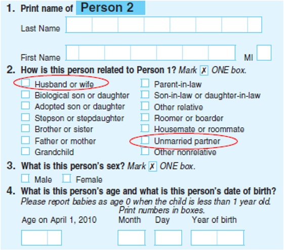
Figure 1. Segment of Questionnaire, 2010 Census of Population, United States. Source: http://2010.census.gov/2010census/pdf/2010_Questionnaire_Info.pdf
Third, a comparison of the data on same-sex partners from the 2010 Census and the 2010 American Community Survey (ACS) showed that “the 2010 Census number of same-sex couple households was 52 percent higher than the ACS estimate” (O’Connell and Feliz, 2011, p. 2).
Owing to the changes between 2000 and 2010 in state marriage laws, as well as to the other issues just mentioned, researchers decided that the newly available 2010 census data on same-sex partnering deserved special methodological attention. The Census Bureau, thus, adjusted the original data from the 2010 census. We now discuss and compare these “original” data from the 2010 Census with the “preferred,” i.e., adjusted by the Census Bureau, data on same-sex couples from the 2010 Census.
According to the officially reported data of the 2010 Census on same-sex partners, referred to here as the “original” data, there were 901,997 same-sex couple households enumerated, representing an increase of 51.8% over the count of same-sex couple households in the 2000 census. By comparison, the total number of households was almost 117 million in 2010, which was an increase of 10.7% from 2000.
Figure 1 shows the portion of the census schedule containing the questions that produced data on same-sex partnered households. The data were based on answers to two different questions, namely, the person’s “relationship to householder,” and the person’s sex. If a person’s relationship to the householder was “unmarried partner” or “husband or wife,” and if the two persons reported the same sex, then the household was classified as a same-sex partner household.
Based on the data produced from these two questions, of the 901,997 same-sex households enumerated in 2010, 552,620 were same-sex households where the persons identified themselves as unmarried partners, and 349,377 were same-sex households where the persons identified themselves as spouses.
When analyzing these data, however, Census Bureau researchers “discovered an inconsistency in the responses in the 2010 Census summary file statistics that artificially inflated the number of same-sex couples … the wrong box may have been checked for the sex of a small percentage of opposite-sex spouses and unmarried partners. Because the population of opposite-sex married couples is large and the population of same-sex married couples in particular is small, an error of this type artificially inflates the number of same-sex married partners. After discovering the inconsistency, Census Bureau staff developed another set of estimates to provide a more accurate way to measure same-sex couple households. The revised figures were developed by using an index of [first, i.e., given] names to re-estimate the number of same-sex married and unmarried partners by the sex commonly associated with the person’s first name” (Bureau of the Census, 2011).
The revised estimates from the 2010 Census, known here as the “preferred” data, indicate that in 2010 there was a total of 646,464 same-sex households, comprised 131,729 same-sex households where the persons identified themselves as spouses, and 514,735 same-sex households where the persons identified themselves as unmarried partners. These “preferred” data from the 2010 Census, by the way, are much closer to the results of the 2010 American Community Survey (ACS) which found 593,324 same-sex households, comprised 152,335 same-sex married couples and 440,989 same-sex unmarried partners.
The preferred same-sex data from the 2010 census “remove from the … counts those couples where the names of the respondents are inconsistent with their reported sex at an index level of 95 percent or more, strongly suggesting that they are opposite-sex couples. [As we have already noted], overall, the total number of same-sex couples declined from 901,997 to 646,464 or by 28 percent. The unmarried partner component declined by 7 percent while the spousal component declined by 62 percent” (O’Connell and Feliz, 2011, p. 27).
The Census Bureau noted in a “News Release” (“Census Bureau Releases Estimates of Same-Sex Married Couples,” 2011) that they distributed their “preferred” estimates to several non-Census Bureau researchers for peer-review; “these experts concluded the methodology behind these revised estimates was sound.”
However, “preferred” estimates for 2010 were only developed by the Census Bureau for the 50 states of the U.S. and for the District of Columbia. “Preferred” estimates of same-sex couples for sub-state areas, e.g., counties, were not developed and published by the Census Bureau. Since our paper focuses on the prevalence of same-sex partnering in metropolitan areas (which are based on counties), we need same-sex partnering data for counties. But “preferred” data for counties produced by the U.S. Census Bureau are not available. Fortunately, Gates, a demographer with the Williams Institute on Sexual Orientation Law and Public Policy at UCLA, has developed a procedure for estimating the numbers of same-sex partners for counties.
Here, now is a summary of the adjustment procedure developed by Gates to develop estimates of the numbers of same-sex male couples and same-sex female couples for counties.
The adjustment procedure (Gates, 2013) involves several steps as follows:
1. For each county, use the mail-in rate to estimate the percentage of different-sex couples who miscoded the sex of a partner or spouse for each county.
where
| g: | the county |
| errorg: | error rate (sex miscoding rate in the county) |
| Mailinpectg: | Percentage of households who used the Census 2010 mail-in survey in the county |
2. Apply the error rate to the official census number of different-sex couples to get the number of miscoded different-sex couples; then subtract it from the census number of same-sex couples in the county to yield a temporary number of same-sex couples.
where
| SSMtg: | temporary number of same-sex male couples in the county |
| SSFtg: | temporary number of same-sex female couples in the county |
| SSMg: | official number of same-sex male couples in the county |
| SSFg: | official number of same-sex female couples in the county |
| DSMARMg: | official number of different-sex married couples with male householder in the county |
| DSUMPMg: | official number of different-sex unmarried couples with male householder in the county |
| DSMARFg: | official number of different-sex married couples with female householder in the county |
| DSUMPFg: | official number of different-sex unmarried couples with female householder in the county |
3. Apply the two temporary variables to create an adjusted proportion of same-sex couples in the counties in the state.
where
| s: | the state |
| adjusted proportion of same-sex couples in the county within the state | |
| adjusted proportion of same-sex female couples in the county within the state | |
| adjusted proportion of same-sex male couples in the county within the state |
If either is negative, the Gates adjustment approach then substitutes a value of zero for the negative value.
4. Apply that proportion to the Census state-level preferred estimates of same-sex couples to develop preferred estimates for the county.
where
| the preferred numbers of same-sex couples in the state | |
| the preferred numbers of same-sex male couples in the state | |
| the preferred estimates of same-sex couples in the county | |
| the preferred estimates of same-sex male couples in the county | |
| the preferred estimates of same-sex female couples in the county |
We have produced a detailed example of the above calculations for one specific county, Anderson County, TX, USA. Readers interested in receiving a copy of the calculations may write to the senior author and request it.
We used the Gates method, as just outlined, to produce numbers of same-sex couples, same-sex male couples and same-sex female couples for each county. Then we used the three numbers for the counties and developed for each of the 366 metropolitan areas of the U.S. in 2010, MSA-level preferred estimates of same-sex couples, same-sex male couples, and same-sex female couples.
However, the Gates adjustment method ends up producing many estimates of zero for same-sex male couples among the counties, thus producing estimates of zero for same-sex male couples in 36 of the 366 metropolitan areas. The Gates method produced counts of same-sex male couples of zero in 36 metropolitan areas. In our view, it is probably not the case that there are no same-sex male couples residing in any of these 36 metropolitan areas.
Therefore, we adjusted the Gates approach by not applying the adjusted proportion of same-sex male couples to the preferred estimates of same-sex male couples for the county level. Instead, we used the numbers of official same-sex male couples and same-sex female couples in the county to recalculate the proportions of same-sex male couples and same-sex female couples in each county. Then applying the two proportions to the county-level preferred estimates of same-sex couples (), we developed preferred estimates for same-sex male couples and same-sex female couples for each county.
To illustrate, we now take a specific metropolitan area that received a zero count of same-sex male couples using the Gates adjusted method, namely, Laredo, TX, USA, and show how we made a different adjustment resulting in a positive value. The Laredo metropolitan area comprises a single county, Webb County. For Webb County, the Gates adjusted method produces an estimate of zero for same-sex male couples, an estimate of 134 for same-sex female couples and, thus, an estimate of 134 for the total number of same-sex couples (). The official census numbers of same-sex male couples and same-sex female couples for Webb County are 156 and 192, respectively. Therefore, the proportions of same-sex male couples and same-sex female couples in Webb County are 0.448 and 0.552. We then applied these proportions to the preferred estimate of same-sex couples for Webb County, namely 134, and thus obtained a count of 60 same-sex male couples and 74 same-sex female couples. Our adjustment differs from that of Gates in that it does not produce any zero counts unless zero counts were actually produced in the official census numbers.
We then use these estimates of the preferred numbers of same-sex male couples and same-sex female couples to calculate our ratios. The method we use is described in the next section.
The Prevalence of Gay and Lesbian Partnering
Earlier research on the prevalence of gay male partners and lesbian partners in different geographic areas of the U.S. (e.g., Gates and Ost, 2004; Walther and Poston, 2004; Baumle et al., 2009; Walther et al., 2011; Gates, 2013) has used several different kinds of rates and ratios to measure the degree of prevalence. Some have been based on individual data on gay male and lesbian partners in which the numbers of gay male partners (or lesbian partners) comprise the numerators, and the numbers of unmarried males (or females) of age 18 and above, or the numbers of married males (or females) of age 18+, or the numbers of all males (or females) of age 18+, comprise the denominators (Walther and Poston, 2004; Baumle et al., 2009; Walther et al., 2011). Rates and ratios have also been developed with household data in which the numbers of gay male (or lesbian) partnered households are the numerators, and the denominators are the numbers of partnered households, or the numbers of all households (Gates and Ost, 2004; Walther and Poston, 2004). An interesting methodological finding in this research is that the various gay male partnering indexes are all highly correlated with one another, as are the various lesbian partnering indexes. The research suggests a certain robustness of the indexes. It does not seem to matter whether persons or households are used as the numerator, or whether ever married, never married, or all persons of age 18 and over, or partnered households or all households are used as the denominator; the variances in the various indexes have been shown to be very similar and, thus, the correlations among and between them are high [for more detail, see Walther and Poston (2004)].
Prevalence Indexes of Gay Male and Lesbian Partnering
In this paper, we develop a household-based index of gay male partnering and a household-based index of lesbian partnering using data for the 366 metropolitan areas of the U.S. Also, as noted above, for comparative purposes, we calculate similar indexes for opposite-sex married couples and opposite-sex cohabiting couples.
The index we develop was first used by Gates and Ost (2004) and by Walther and Poston (2004). The index is a “ratio of the proportion of same-sex couples living in a [metropolitan area] to the proportion of households that are located in a [metropolitan area]… This ratio … measures the over- or underrepresentation of same-sex couples in a geographic area relative to the population” (Gates and Ost, 2004, p. 24). An index value of 1.0 for a metropolitan area indicates that “a same-sex couple is just as likely as a randomly picked household to locate” in the metro area (Gates and Ost, 2004, p. 24). An index value above 1.0 means that a same-sex couple is more likely to live in the metro area than a random household, and a value less than 1.0, less likely. The formula for the ratio is as follows:
Where : i = metro area
Table 1 presents descriptive data for the ratios for gay male couples and lesbian couples among the 366 metropolitan areas in 2010, along with the descriptive data for opposite-sex married couples and opposite-sex cohabiting couples. See Table S1 in Supplementary Material for each of the four ratios for each of the 366 metropolitan areas.
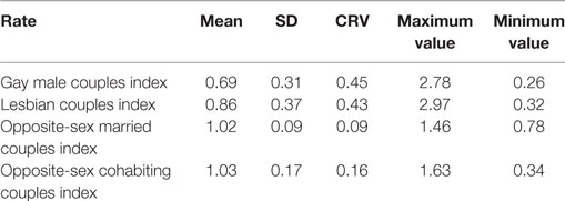
Table 1. Means, SD, coefficients of relative variation (CRV), and minimum and maximum values: ratios of gay male couples and lesbian couples, and ratios of opposite-sex married couples and opposite-sex cohabiting couples: 366 Metropolitan Areas of the U.S., 2010.
The mean across the 366 metropolitan areas for gay male households is 0.69 and is 0.86 for lesbian households. This means that, in the “average” metropolitan area, gay male couples are 31% less likely to settle there than would be a couple from a randomly selected metropolitan household; and that a lesbian couple would 14% less likely to settle there than would be a couple from a randomly selected household.
We show in Table 2 that the San Francisco–Oakland–Fremont, CA metropolitan area (hereafter referred to as San Francisco) has the highest gay male couple ratio value, 2.78, and the Ithaca, NY metropolitan area has the highest lesbian couple index ratio, 2.97. The value for the San Francisco area may be interpreted as indicating that a gay male couple is 2.8 times more likely than an “average” couple in a U.S. metro household to reside in the San Francisco area, or, in other words, 180% more likely [that is (2.78 − 1.00) × 100]. The Ithaca index value indicates that a lesbian couple is almost 200% more likely to live in Ithaca than an average couple in a U.S. metro household is likely to live in Ithaca.
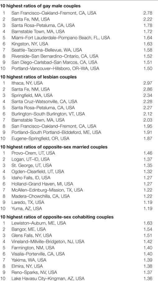
Table 2. Ten highest ratios of gay male couples, lesbian couples, opposite-sex married couples, and opposite-sex cohabiting couples: 366 metropolitan areas, USA, 2010.
Regarding the lowest ratios (Table 3), the Grand Forks, ND–MN metro area has the lowest gay male couple ratio, 0.26, and the Wausau, WI has the lowest lesbian couple ratio, 0.32. Gay male couples are about one-quarter as likely (or 74% less likely) to live in Grand Forks as a randomly picked U.S. metro household, and lesbian couples are about one-third as likely to live in Wausau as a randomly selected household.
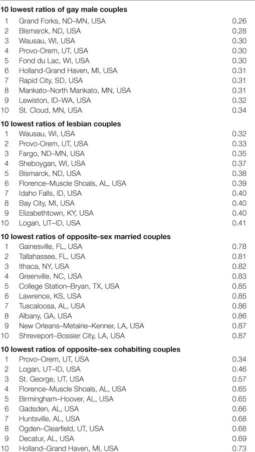
Table 3. Ten lowest ratios of gay male couples, lesbian couples, opposite-sex married couples and opposite-sex cohabiting couples: 366 metropolitan areas, USA.
For comparative purposes, we also present in Table 1 descriptive data for ratios for opposite-sex couples. The average metropolitan area has a ratio value of 1.02 for opposite-sex married couples, and a ratio of 1.03 for opposite-sex cohabiting couples. This means that the average metro area is just about as likely to have an opposite-sex married couple or an opposite-sex cohabiting couple residing there as it would be likely to have a randomly selected couple from a metro household residing there. Of all the metro areas, the Provo–Orem, UT area is the most likely to have an opposite-sex married couple located there, with a ratio value of 1.46. And the Lewiston–Auburn, ME area is the most likely of all the metro areas to have an opposite-sex cohabiting couple residing there (Table 2). The metro areas with the lowest opposite-sex ratios are the Gainesville, FL metro area with an opposite-sex married couples value of 0.78, and the Provo–Orem, UT area with an opposite-sex cohabiting couples ratio of 0.34 (Table 3).
Table 2 reports the 10 highest ratios and Table 3 the 10 lowest ratios for same-sex male and lesbian partnering. Five metro areas are among the top 10 areas for both the gay male and lesbian ratios. There are also some similarities among the metro areas with respect to the lowest gay male and lesbian ratios (Table 3), but there are not as many metro areas among the 10 with the lowest values as there are among the 10 with the highest values, 3 versus 5.
Variation in the Four Partnering Ratios Across the Metropolitan Areas
We now compare the degree to which these four sets of partnering indexes (gay males, lesbians, opposite-sex married, and opposite-sex cohabiting) vary across the 366 metropolitan areas. Since the means for the four ratios are very different (see Table 1), we should not compare their respective SDs. The third data column of Table 1 presents values for the four partnering ratios of the coefficient of relative variation (CRV = SD divided by the mean), a normalized measure of dispersion. The CRV is especially useful and preferred over the straightforward SD when one wishes to compare the levels of dispersion of data with different means.
The CRVs for the two same-sex ratios are 0.45 and 0.43, i.e., they are very similar; the CRV for the opposite-sex cohabiting index is almost one-third as large at 0.16, and the CRV for the opposite-sex married index is even lower, at 0.09. As one might expect, there is clearly much greater relative variation across the metro areas in both of the same-sex partnering indexes, with the opposite-sex cohabiting index values having the next highest amount of relative variation, and the opposite-sex married index values showing the lowest amount.
Comparison of Ratios for Gay Male Partners with the Ratios for Lesbian Partners
Past research on the geographic locations of same-sex partners (see, e.g., Gates and Ost, 2004; Baumle et al., 2009; Walther et al., 2011; Gates, 2013) has shown for the most part that across geographical areas the prevalence indexes of gay males and lesbians are positively related, but that lesbian partners tend to have higher prevalence indexes in most geographical areas than gay male partners. In Figure 2, we present a scatterplot comparing for the 366 metropolitan areas in 2010 the prevalence indexes for gay male partners with those for lesbian partners. The diagonal line in the figure is not a regression line, but, rather, a line representing equal gay male and lesbian partnering ratio index values. Observations above the diagonal line refer to areas with higher gay male ratios than lesbian ratios; and vice versa for observations below the line.
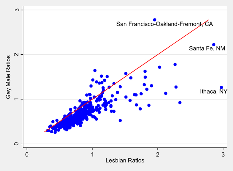
Figure 2. Scatterplot comparing ratio index values for gay male couples with ratio index values for lesbian couples: 366 metropolitan areas of the U.S., 2010.
We see in Figure 2 evidence of a clear positive relationship between the gay male ratios and the lesbian ratios; r = 0.81. However, we also see in Figure 2 that in most metropolitan areas the prevalence ratios for lesbian partners are higher than those for male partners. That is, most of the metropolitan areas are located below the diagonal line in Figure 2, meaning that their lesbian ratios are greater than their gay male ratios. To illustrate, we have identified by name the observation for the Ithaca metro area; its lesbian ratio is 2.97, and its gay male ratio is 1.26. Also identified in Figure 2 is the Santa Fe area, with a lesbian ratio of 2.86 and a gay male ratio of 2.22. By contrast, the San Francisco metro area has a gay male ratio of 2.78, much higher than its lesbian ratio of 1.95.
In all, of the 366 metropolitan areas, 328 (or almost 90%) of them have higher lesbian ratios than gay male ratios. Among the 38 metro areas with higher gay male than lesbian ratios, many are typically large, cosmopolitan, expensive, and well-established areas, such as San Francisco, Miami, Seattle, San Diego, Washington, DC, Las Vegas, Los Angeles, Atlanta, Denver, New York, Tampa, Phoenix, Dallas, New Orleans, Honolulu, Chicago, and Houston. [In an analysis we conducted using 2000 census data, we found a very similar result, that is, the prevalence indexes were higher for lesbians than for gay males in 92% of the metro areas (Walther et al., 2011).]
We noted above the very high correlation between the gay male ratios and the lesbian ratios; this means that gay and lesbian couples tend to settle in similar metropolitan areas, although not at the same levels. Indeed in almost 90% of the metropolitan areas the levels of lesbian prevalence are greater than the levels of gay prevalence. Gay males, thus, appear to have a few favorite metropolitan areas, namely San Francisco, Atlanta, Los Angeles, Miami, Washington, DC, New York, Houston, and the other areas mentioned above where their prevalence ratios surpass those of lesbians. Partnered lesbians, on the other hand, tend to have concentrations that are greater than those of gay males in most of the metropolitan areas, tending not to prefer certain metropolitan areas to the degree they are preferred by gay males.
Correlates of Gay Male and Lesbian Partnering in the Metropolitan Areas of The U.S.
We turn now to the issue of accounting for variation in the indexes of gay male and lesbian partnering. Among the metropolitan areas, why, for instance, do San Francisco and Miami have the highest gay male partnering indexes, and why do Ithaca and Santa Fe have the highest lesbian ratios (see Table 2)? Why do Grand Forks and Bismarck have the lowest gay male partnering ratios, and why do Wausau and Provo–Orem have the lowest lesbian ratios (see Table 3)? What kinds of social and ecological characteristics of the metropolitan areas might be brought to bear to answer these questions? In this section, we draw on sociological human ecology and a literature dealing with gay and lesbian settlement patterns to identify characteristics of metropolitan areas that one could be related to levels of gay male and lesbian concentration; we then propose and test a number of hypotheses in an attempt to address this issue.
The size of the metropolitan area’s total population should be associated in a positive way with the levels of gay male and lesbian concentration. There is good reason to expect higher levels of gay and lesbian concentration in areas with larger populations (Abrahamson, 2002; Gates and Ost, 2004; Walther et al., 2011). These expectations are based in part on the notion that the larger the size of the general population, the greater the likelihood for some of the residents to be gay males and lesbians.
Also, we have reason to expect that levels of gay male and lesbian concentration should be positively associated with levels of heterosexual cohabitation. If the social and political climate of a metropolitan area is conducive to heterosexual cohabitation, then one might argue that the same should be the case for homosexual cohabitation (Black et al., 2002; Florida, 2002, 2005; Walther et al., 2011). Metro areas that are more accepting of heterosexual unmarried couples who are living together should be more accepting of gay males and lesbians living together. These so-called more accepting populations will likely be politically and socially more liberal, or less conservative, than populations less accepting of heterosexual cohabitants. Metro areas with large college populations, e.g., Ithaca, NY, USA and Eugene, OR, USA, will be more social and politically liberal, and more accepting of men and women living together without being married; we expect such places will also be more accepting of same-sex cohabitation. Thus, metropolitan areas with a high prevalence of unmarried heterosexuals who are cohabiting should have a high prevalence of homosexual cohabitation, and vice versa.
We also hypothesize that the median age of the population in the metro area should be associated in a negative manner with levels of gay male and lesbian concentration. Given that much older populations tend to be more conservative than younger populations, we expect that the higher the median age of the population, the lower the level of same-sex partnering (Florida, 2002, 2005).
We also expect that the mode of household occupancy should be associated with the prevalence of same-sex partnering. Among the metropolitan areas, we hypothesize that the higher the percentage of households that are renter occupied, the higher the prevalence of gay male and lesbian partnering. This hypothesis is based in part on the fact that rental housing tends to be more associated with a more mobile and dynamic, i.e., politically and socially liberal, populations that would be more receptive to same-sex partnering than populations characterized by high levels of owner-occupied housing, which are typically more permanent and perhaps staid and conservative (Hawley, 1950; Poston and Frisbie, 1998, 2005).
Finally, we expect that the higher the percentages of African Americans and Latinos in the populations, the larger the presence of same-sex partnering. This expectation is based in part on the fact that same-sex partners are themselves a minority population – albeit sexual and not racial/ethnic – and will tend to be more concentrated in areas with proportionally larger, rather than smaller, numbers of racial and ethnic minorities (Hawley, 1950; Poston and Frisbie, 2005).
The first two columns of Table 4 present the results of two ordinary least squares (OLS) multiple regression equations modeling the prevalence of gay male partners and lesbian partners among the 366 metropolitan areas. We have placed positive or negative signs to the right of the name of each independent variable indicating the direction of the variable’s hypothesized relationship with the gay male (or lesbian) household index ratios.
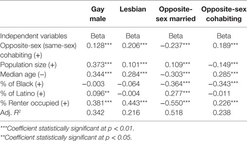
Table 4. Standardized regression coefficients from four multiple regression equations of same-sex gay male partnering ratios, same-sex lesbian partnering ratios, opposite-sex married partnering ratios, and opposite-sex cohabiting partnering ratios, on six independent variables: 366 metropolitan areas of the U.S., 2010.
We note first that the statistical tolerances of the six independent variables are all acceptable. In the gay male and lesbian equations, the tolerances range from a low of 0.53 (percentage renter occupied) to a high of 0.88 (population size). The mean tolerance of the six independent variables in the metro area equations is 0.68. Multicollinearity does not appear to be an issue in any of the equations presented in Table 4.
Looking at the standardized regression coefficient results across the metropolitan areas predicting levels of gay male concentration (left panel of data of Table 4), four are signed in the hypothesized direction, and all four of them are statistically significant. The larger the concentration of renter-occupied housing, and the larger the percentage of Latinos in the metropolitan area, the higher the gay male partnering ratio. Also, the higher the prevalence of unmarried cohabitation and the larger the population size, the higher the gay male partnering ratio. The median age variable, however, is related positively, not negatively as hypothesized, with same-sex male prevalence. And the percentage Black variable is not signed as hypothesized, and it is also not statistically significant. The renter variable has the largest standardized coefficient; for every one SD increase in the percentage of the metro area population in rental housing, there is a 0.38 SD increase in the gay male concentration ratio, holding constant the effects of the other independent variables. The population size variable has the next strongest effect on the gay male ratio.
We next look at the regression results predicting among the 366 metropolitan areas the prevalence of lesbian partnering. With only one difference from the results for the gay male equation, those for the lesbian equation are the same. The higher the prevalence of unmarried cohabitation and the larger the population size, the higher the lesbian partnering ratio. And the larger the concentration of renter-occupied housing in the metro area, the higher the lesbian partnering ratio. Also, as was the situation in the gay male equation, the renter variable has the strongest relative effect on the lesbian partnering ratio of all six independent variables. For every one SD increase in the rental housing variable, there is a 0.44 SD increase in the lesbian partnering ratio, holding constant the effects of the other independent variables.
For comparative purposes, we now turn to analyses of heterosexual partnering among the 366 metropolitan areas, specifically that involving opposite-sex married couples and opposite-sex cohabiting couples. We first ask whether the variability among the 366 metropolitan areas in each of the two homosexual partnering ratios is related to the variability in each of the two heterosexual partnering ratios. One might expect that metro areas with high levels of homosexual partnering (either gay male or lesbian) should also have high levels of heterosexual cohabitation. After all, as we noted earlier, if the climate of a metropolitan area is conducive to gay male or lesbian cohabitation, the same should be the case for heterosexual cohabitation.
Table 5 reports the zero-order correlations between each of the opposite-sex partnering ratios and each of the same-sex partnering ratios. We noted above that the correlation between the two same-sex ratios is positive and very high: r = 0.81. But this is not the situation for the correlations between either of the opposite-sex ratios and either of the same-sex ratios. We had expected that the opposite-sex cohabiting ratio would be positively and highly correlated with both of the same-sex ratios. While it turns out that the two correlations are positive, they are not very high; the correlation between the opposite-sex cohabiting ratio and the same-sex gay male ratio is 0.18, and that between the opposite-sex cohabiting ratio and the same-sex lesbian ratio is 0.29. And the correlations between the opposite-sex married ratio and the two same-sex ratios are both negative. The variation in the ratios is not at all similar when comparing the opposite-sex ratios with the same-sex ratios (Table 5). This leads us to suspect, thus, that the kinds of independent variables that are most related to either of the same-sex ratios (as discussed several paragraphs earlier) will not be the same as those most highly related to either of the opposite-sex ratios.
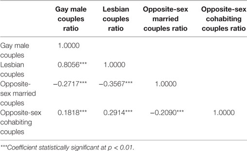
Table 5. Matrix of zero-order correlations between each pair of four partnering ratios: same-sex gay male partnering ratios, same-sex lesbian partnering ratios, opposite-sex married partnering ratios, and opposite-sex cohabiting partnering ratios: 366 metropolitan areas of the U.S., 2010.
We present in the third and fourth columns of Table 4 the results of two OLS regression equations predicting variation in the ratios for opposite-sex married couple (third column) and for opposite-sex cohabiting couples (fourth column). The same independent variables used in the homosexual equations are used here in the heterosexual equations, with one exception; the first independent variable in the opposite-sex equations refers to homosexual partnering (male–male households plus female–female households) rather than to opposite-sex partnering.
The regression results in Table 4 predicting variation in the opposite-sex ratios (columns 3 and 4) are different from those predicting variation in the same-sex ratios (columns 1 and 2). Regarding the opposite-sex cohabiting equation, the population size, percentage Black and percentage Latino independent variables are negatively, not positively, signed. And regarding the opposite-sex married equation, the cohabitation, percentage Black, and the rental independent variables are negatively, not positively, signed. And in this equation, the median age variable is signed negatively as hypothesized; in all the other equations, it is positively signed. In summary, the regression results of the two heterosexual equations are more different from, than similar to, the regression results of the two homosexual equations. The statistically important and significant effects in the two heterosexual equations differ somewhat from those in the homosexual equations. This suggests that factors explaining variation in the homosexual equations and not always the same as those in the heterosexual equations. We conclude our paper with a general discussion of these results.
Discussion and Conclusion
In this paper, we used recently released and statistically adjusted data from the 2010 Census to analyze patterns of gay male partnering and lesbian partnering in the metropolitan areas of the U.S. A key concern with the 2010 census data on same-sex partnering is the quality of the data. When Census Bureau researchers first began to analyze the data, they discovered an error that produced an artificial inflation of the number of same-sex partners; some of the respondents apparently checked the wrong box for the census question asking about their sex. Census Bureau staff, hence, developed a set of adjusted data, known as the “preferred” data, which better reflected the true number of same-sex couple households. But the Census Bureau only produced the “preferred” estimates for the states of the U.S. The demographer, Gary Gates developed an algorithm to develop estimates at the county level. We used in this paper the Gates method, but we revised it slightly to address the fact that the Gates method often produced zero counts, usually for same-sex male couples, for the smaller geographic areas. We made an adjustment in the Gates method to minimize the likelihood of zero counts.
Regarding our results, the San Francisco area was shown to have the highest same-sex gay male prevalence ratio, and the Ithaca area the highest same-sex lesbian ratio. We showed that among the metro areas the gay male partnering ratios and the lesbian partnering rates were highly and positively correlated. Owing to these positive correlations, we concluded that gay male households and lesbian households tend to be concentrated in similar metro areas, although not at the same levels. Indeed, we showed that in most of the metro areas, the levels of lesbian partnering were greater than the levels of gay male partnering. In almost 90% of the 366 metro areas, the lesbian ratio was larger in magnitude than the gay male ratio. Gay males seem to have a few favorite metropolitan areas, namely, San Francisco, Atlanta, Los Angeles, Miami, Washington, DC, New York, Houston, and some others where their prevalence ratios surpass those of lesbians. Partnered lesbians, on the other hand, have concentrations that are greater than those of gays in most of the metropolitan areas, tending not to prefer certain metropolitan areas to the degree they are preferred by gay males.
Finally, we estimated multiple regression equations predicting gay male partnering and lesbian partnering among the metro areas. And for comparative purposes, we estimated similar regression equations predicting opposite-sex cohabiting partnering and opposite-sex married partnering. We were concerned here with ascertaining the kinds of structural characteristics that influence and are related to the geographical locations of gay male and lesbian partners. Drawing on sociological human ecology and a more limited literature dealing with gay and lesbian settlement patterns, we identified several characteristics of metropolitan areas that could be argued to be related to levels of gay male and lesbian partnering concentration.
In the multivariate context, the variables shown to be most influential in predicting levels of gay and lesbian concentration were a variable capturing the degree of prevalence of rental housing, a variable measuring the population size of the area, and a measure of heterosexual cohabitation. We need to further our research predicting levels of gay male and lesbian partnering. One avenue for future research would involve developing same-sex partnering indexes for the metro areas for racial and ethnic groups, that is, for non-Hispanic whites, non-Hispanic blacks, and Hispanics. We might also develop same-sex partnering indexes that distinguish the populations by two or more broad age groups. The multivariate analyses reported here are just beginning to address the question of why some metropolitan areas have high same-sex partnering rates and why other areas have low rates.
This paper has undertaken a quantitative examination of the prevalence of partnered gay male and partnered lesbian households in the metropolitan areas of the U.S. in 2010. It builds on and extends the previous and limited literature on the prevalence of gay males and lesbians in geographical areas of the U.S. (Black et al., 2000, 2002; Gates and Ost, 2004; Walther and Poston, 2004; Baumle et al., 2009; Walther et al., 2011; Gates, 2013).
Quantitative assessments of the patterns of gay and lesbian prevalence in U.S. metropolitan areas are particularly relevant today given the active discussions in the political, religious, and social arenas with regard to homosexual marriage, the adoption of children by gays and lesbians, and other issues involving sexual orientation. As Gates and Ost (2004) (p. 3) have written, these topics lead to intense discussions, arguments, and debates, most of which are “marked by an astonishing lack of empirical data.” It has been difficult if not impossible for policymakers, community activists, and gay and lesbian leaders to appraise the effects that homosexual marriage laws, domestic partnership benefits, adoption rights, and other related issues would have on the homosexual and heterosexual communities in the country because of the paucity of information about the locations of gays and lesbians. Aside from everyone seeming to know that there are a lot of homosexuals in San Francisco, the amount of knowledge about the prevalence of gay males and lesbians elsewhere in the U.S. is miniscule. It is hoped that the quantitative analyses of 2010 census data presented in this paper will contribute toward addressing this void.
Author Contributions
DP wrote the bulk of the article and conducted most of the analysis. YC assisted in the statistical analysis and the writing of the article.
Conflict of Interest Statement
The authors declare that the research was conducted in the absence of any commercial or financial relationships that could be construed as a potential conflict of interest.
The reviewer MD and handling Editor declared their shared affiliation, and the handling Editor states that the process nevertheless met the standards of a fair and objective review.
Supplementary Material
The Supplementary Material for this article can be found online at https://www.frontiersin.org/article/10.3389/fsoc.2016.00012
References
Barrett, R. E. (1994). Using the 1990 U.S. Census for Research. Thousand Oaks, CA: SAGE Publications.
Baumle, A. K., Compton, D., and Poston, D. L. Jr. (2009). Same-Sex Partners: The Social Demography of Sexual Orientation. New York: SUNY Press.
Baumle, A. K., and Poston, D. L. Jr. (2011). The economic cost of homosexuality: multilevel models. Soc. Forces 89, 1005–1032. doi: 10.1093/sf/89.3.1005
Black, D. A., Gates, G., Sanders, S. G., and Taylor, L. J. (2000). Demographics of the gay and lesbian population in the United States: evidence from available systematic data sources. Demography 37, 139–154. doi:10.2307/2648117
Black, D. A., Gates, G., Sanders, S. G., and Taylor, L. J. (2002). Why do gay men live in San Francisco? J. Urban Econ. 51, 54–76. doi:10.1006/juec.2001.2237
Bureau of the Census. (2011). Census Bureau Releases Estimates of Same-Sex Married Couples. Washington, DC: Bureau of the Census.
Fields, J., and Clark, C. L. (1999). “Unbinding the ties: edit effects of marital status on same gender couples,” in Population Division Working Paper No. 34, Fertility and Family Statistics Branch (Washington, DC: U.S. Census Bureau).
Florida, R. (2002). The Rise of the Creative Class: And How It’s Transforming Work, Leisure, Community, & Everyday Life. New York, NY: Basic Books.
Florida, R. (2005). The Flight of the Creative Class: The New Global Competition for Talent. New York, NY: Harper Collins.
Gates, G. J. (2010). Same-Sex Couples in the U.S. Census Bureau Data: Who Gets Counted and Why. Los Angeles, CA: The Williams Institute.
Gates, G. J. (2013). “Geography of the LGBT population,” in International Handbook on the Demography of Sexuality, ed. A. K. Baumle (New York, NY: Springer), 229–242.
Gates, G. J., and Ost, J. (2004). The Gay and Lesbian Atlas. Washington, DC: The Urban Institute Press.
O’Connell, M., and Feliz, S. (2011). “Same-sex couple household statistics from the 2010 census,” in Working Paper Number 2011–26 (Washington, DC: U.S. Census Bureau, Social, Economic and Housing Statistics Division).
O’Connell, M., and Gooding, G. (2006). “The use of first names to evaluate reports of gender and its effect on the distribution of married and unmarried couple households,” in Paper presented at Population Association of America Annual Meeting. Los Angeles, CA.
O’Reilly, K., and Webster, G. R. (1998). A sociodemographic and partisan analysis of voting in three anti-gay rights referenda in Oregon. Prof. Geogr. 50, 498–515. doi:10.1111/0033-0124.00135
Poston, D. L. Jr., and Frisbie, W. P. (1998). “Chapter 2 human ecology, sociology, and demography,” in Continuities in Sociological Human Ecology, eds M. Micklin and D. L. Poston Jr. (New York: Plenum Press), 27–50.
Poston, D. L. Jr., and Frisbie, W. P. (2005). “Chapter 20 ecological demography,” in Handbook of Population, eds D. L. Poston Jr. and M. Micklin (New York, NY: Springer Publishers), 601–623.
Simmons, T., and O’Connell, M. (2003). “Married couple and unmarried-partner households: 2000,” in Census 2000 Special Reports. CENSR-5 (Washington, DC: U.S. Bureau of the Census).
Virgile, M. (2011). Measurement Error in the Relationship Status of Same-Sex Couples in the 2009 American Community Survey: Final Report. Washington, DC: U.S. Census Bureau, American Community Survey Research and Evaluation Program.
Walther, C. S., and Poston, D. L. Jr. (2004). Patterns of gay and lesbian partnering in the larger metropolitan areas of the United States. J. Sex Res. 41, 201–214. doi:10.1080/00224490409552228
Keywords: gay male, lesbian, same sex, census, metropolitan area, human ecology
Citation: Poston DL Jr and Chang Y-T (2016) Patterns of Gay Male and Lesbian Partnering in the Metropolitan Areas of the United States in 2010. Front. Sociol. 1:12. doi: 10.3389/fsoc.2016.00012
Received: 01 February 2016; Accepted: 19 July 2016;
Published: 02 August 2016
Edited by:
Anna Rotkirch, Population Research Institute, Väestöliitto, FinlandReviewed by:
Mirkka Danielsbacka, Population Research Institute, Väestöliitto, FinlandTrond Viggo Grøntvedt, Norwegian University of Science and Technology, Norway
Copyright: © 2016 Poston and Chang. This is an open-access article distributed under the terms of the Creative Commons Attribution License (CC BY). The use, distribution or reproduction in other forums is permitted, provided the original author(s) or licensor are credited and that the original publication in this journal is cited, in accordance with accepted academic practice. No use, distribution or reproduction is permitted which does not comply with these terms.
*Correspondence: Dudley L. Poston Jr., d-poston@tamu.edu