Forward Modeling of EUV and Gyrosynchrotron Emission from Coronal Plasmas with FoMo

1. Introduction

The mean free path of photons becomes increasingly long when going up from the solar photosphere, into the solar corona. Thus, the solar corona is typically optically thin. As a result, observations are 2D projections of a 3D configuration in the solar corona. This makes interpreting observations rather difficult, because the precise position of the plasma along the line-of-sight (LOS) is unavailable. One exception is stereoscopy with the STEREO space mission (e.g., Marsh et al., 2009; Verwichte et al., 2009; Aschwanden, 2011), where one uses multiple vantage points to infer the 3D structure of the observations.

The lack of 3D information in observations also makes the comparison of simulation or model data to observations difficult. Typically, simulations output physical quantities in the plasma that cannot be measured directly (e.g., density, temperature), while observations only show spectral line profiles (integrated over space, time and wavelength, depending on the instrument). Thus, to allow for a direct comparison, a conversion from model data to emission is necessary by creating artificial observations. This technique is called forward modeling.

In solar coronal physics, several tools are available for forward modeling. Perhaps the most prominent one is FORWARD, which computes EUV emission and polarimetric signals from a given coronal model (Gibson, 2015; Gibson et al., 2016). Besides that, there is the GX_SIMULATOR (Nita et al., 2015), which computes radio and X-ray emission and is mainly aimed at forward modeling flares. In this article, we will describe the technical aspects of the FOMO tool, another possibility for calculating coronal emission, mainly developed at the KU Leuven (Belgium).

The development of the FOMO tool was mainly motivated by the desire to perform forward modeling of coronal wave models. It had become clear that the connection between wave properties and the expected emission was less straightforward than expected. For instance, Gruszecki et al. (2012) used a naive forward modeling method (i.e., putting the emission in each simulation point proportional to $n_e^2$, where n_e is the electron density) to show that the intensity modulation of sausage waves (e.g., Vasheghani Farahani et al., 2014) is second order in the wave amplitude, because the density depletion is compensated in first order by the increased LOS. FOMO was thus first used by Antolin and Van Doorsselaere (2013) to calculate the emission from numerical and analytical models of the sausage mode, in a self-consistent way using atomic data from the CHIANTI database (Dere et al., 1997; Landi et al., 2013). Antolin and Van Doorsselaere (2013) showed that the sausage mode causes EUV intensity variations, but that the level of variation is highly dependent on the temperature of the emitting loop and the spectral line, the observational setup and instrument (LOS angle and instrument resolution).

After extending FOMO in order to compute gyrosynchrotron emission, Reznikova et al. (2014) compared the full, integrated emission from sausage modes in a cylindrical model to the analytical predictions and found that the predicted phase was not valid (e.g., Mossessian and Fleishman, 2012), although only a uniform distribution of non-thermal particles in the loop was considered. Kuznetsov et al. (2015) extended the model to a 3D semi-torus loop, and Reznikova et al. (2015) computed the expected polarization variations for sausage modes.

The FOMO code was also used for modeling the emission from propagating slow waves. On the one hand, it was used to model the emission features of slow waves and periodic upflow (if such a thing exists in MHD) by De Moortel et al. (2015). It was found that these two physical behaviors are almost impossible to distinguish observationally. On the other hand, FOMO was used to model the damping behavior of slow waves. Previously, it had been found that omnipresent slow waves (Krishna Prasad et al., 2012) had a peculiar dependence of the damping length on the period (Krishna Prasad et al., 2014). With FOMO, it was shown that this behavior could be explained by damping with thermal conduction (Mandal et al., 2016). Furthermore, the propagating slow waves in hot coronal loops (Kumar et al., 2013, 2015) were modeled successfully with FOMO (Fang et al., 2015). Additionally, FOMO was used for the modeling of standing slow waves in hot coronal loops (Wang, 2011; Yuan et al., 2015).

Last but not least, we mention the modeling of standing kink waves in coronal loops performed with FOMO. Antolin et al. (2014, 2015) have calculated the emission from a 3D simulation of a transversally oscillating coronal loop and prominence. In the former work, it was argued that the Kelvin-Helmholtz instability in the resonant layer around the loop could lead to the formation of apparently stranded loops. The simulations in the latter work were used to compare to observational results (Okamoto et al., 2015). The excellent agreement and the direct comparison between the observational signatures and forward model from the simulation allowed to identify the observations as a signature of resonant absorption.

It is clear from the above description that FOMO is ideally situated to improve the current coronal seismology techniques. Coronal seismology compares observations of coronal waves to their models, in order to obtain extra information on the plasma background (such as a coronal loop). For a review on coronal seismology, please see e.g., Nakariakov and Verwichte (2005); De Moortel and Nakariakov (2012); Liu and Ofman (2014). In particular, coronal seismology may be used for the measurement of the magnetic field (e.g., Nakariakov and Ofman, 2001; Van Doorsselaere et al., 2007) and, in general, Alfvén travel times (Arregui et al., 2007; Goossens et al., 2008; Asensio Ramos and Arregui, 2013). Thus, by allowing a direct comparison between the observations and the forward modeling, FOMO improves the magnetometry by waves in the solar corona (i.e., by coronal seismology).

Furthermore, while FOMO is targeted at modeling emission from coronal plasma, its use can be extended to the calculation of emission from any optically thin medium.

2. Forward Modeling with FoMo

2.1. General Approach

In what follows, three numerical implementations of the forward modeling procedure will be described: FOMO-C, FOMO-IDL, FOMO-GS. First, FOMO-IDL was developed to model the EUV emission of the solar corona. A little while later, FOMO-GS was written to extend its application to the gyrosynchrotron radiation. It became clear that IDL is not widely available on clusters, and therefore it was decided to also implement the procedure in C++ (FOMO-C), immediately also giving access to parallelization. In this paragraph, we first describe what is common in all three implementations.

The corona is optically thin, and thus the specific intensity I(λ, x′, y′) (in ergs cm⁻² s⁻¹ sr⁻¹ Å⁻¹) at a wavelength λ is the integral of the monochromatic emissivity ϵ(λ, x, y, z) at each point along the LOS. Let us assume that the LOS is along a given z′ axis, that may not be aligned to any of the numerical axes.

$\begin{array}{ll}I(\lambda ,x\prime ,y\prime )=\int ϵ(\lambda ,x(z\prime ),y(z\prime ),z(z\prime ))dz\prime .& (1)\end{array}$

Here (x, y, z) are the coordinates in the original simulation, and (x′, y′, z′) are the coordinates in the rotated frame of reference of the observation. (x′, y′) are the coordinates in the image plane (also known as the plane-of-the-sky, or POS), and z′ is the direction along the LOS. The two coordinate systems are connected by two rotations, first an angle l around the z-axis, then around an angle −b around the y-axis:

$\begin{array}{cc}\left(\begin{array}{c}x\prime \\ y\prime \\ z\prime \end{array}\right)=\left(\begin{array}{ccc}\cos b& 0& -\sin b\\ 0& 1& 0\\ \sin b& 0& \cos b\end{array}\right)\left(\begin{array}{ccc}\cos l& -\sin l& 0\\ \sin l& \cos l& 0\\ 0& 0& 1\end{array}\right)\left(\begin{array}{c}x\\ y\\ z\end{array}\right).& (2)\end{array}$

The simulation box with grid (x, y, z) is considered as the input for FOMO, and is the data for which the forward model needs to be computed. FOMO-C and FOMO-IDL calculate the optically thin EUV emission in spectral lines or AIA passbands. There the input model needs to contain the x−, y−, z−coordinates of each data point, and specify the number density n_e, the temperature T and three velocity components (v_x, v_y, v_z) at these data points. For the necessary input of the FOMO-GS code, please see Section 2.4.

Then, a new grid is generated in the observation reference frame (x′, y′, z′). The grid points in this new, “observational” grid are called voxels. The resolution of the new grid is set by the user in FOMO-C, and determined from the simulation grid in FOMO-IDL and FOMO-GS. In FOMO-C, the choice for the resolution in the z′−direction (Δl) should be close to the numerical resolution of the input model, as otherwise emission features may be missed in the forward models.

The numerical resolution of the forward model is not related to the instrument resolution. The numerical resolution is necessary to capture the fine emission features that may be present in the numerical model. The instrument resolution should be simulated by post-processing the forward model with a point spread function (or simply summing pixels to degrade the image).

At each voxel $(x_i^{\prime },y_j^{\prime },z_k^{\prime })$, the emissivity is interpolated from the nearest grid point in the (x, y, z)-space and then the LOS integration is performed. The configuration is schematically shown in Figure 1. The integral in Equation (1) is then discretised as follows

$\begin{array}{ll}I(\lambda ,x_i^{\prime },y_j^{\prime })={\displaystyle \sum _k}ϵ(\lambda ,x_i^{\prime },y_j^{\prime },z_k^{\prime })\Delta l,& (3)\end{array}$

which converges to the true emission for Δl → 0, thus stressing the need for a high resolution in the z′−direction in FOMO-C. The FOMO-GS code additionally computes the radiative transfer along the LOS because it is optically thick, and thus the computation is more complicated (see Section 2.4).

FIGURE 1

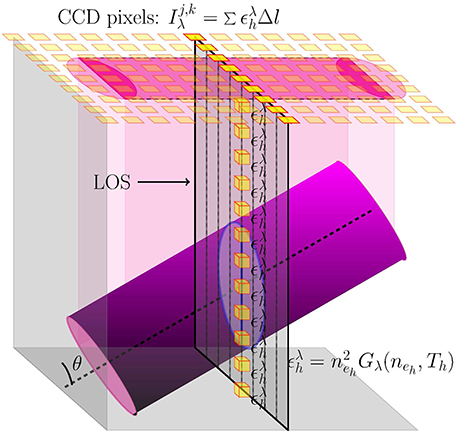
Figure 1. A schematic representation of the LOS through the simulation box in FoMo. The yellow boxes are the voxels along a specific LOS. Figure taken from Yuan et al. (2015).

For calculation of monochromatic emission with FOMO-C and FOMO-IDL, we first convert the physical variables n_e, T to the emissivity $\widetilde{ϵ}(x,y,z)$ (in ergs cm⁻³ s⁻¹ sr⁻¹) of the spectral line at rest wavelength λ₀ at each grid point by

$\begin{array}{ll}\widetilde{ϵ}(x,y,z)=\frac{A_b}{4\pi }{n}_e^2(x,y,z)G_{{\lambda }_0}(n_e(x,y,z),T(x,y,z)),& (4)\end{array}$

where A_b is the abundance of the emitting element (with respect to hydrogen) and $G_{{\lambda }_0}$ the contribution function for that specific spectral line (including the Gaunt factor and oscillator strength for the spectral line). The abundance A_b is taken to be constant along the LOS. The abundance A_b is read from a CHIANTI abundance file. As a standard sun_coronal.abund is used in FOMO-C and FOMO-IDL, but it may be swapped with another file if needed.

The $G_{{\lambda }_0}$ is calculated by a look-up table. The look-up table was generated for a range of temperatures and densities using g_of_t.pro in the CHIANTI database (Dere et al., 1997; Landi et al., 2013). This routine assumes that the plasma satisfies the coronal approximation, in particular, that electrons and protons have the same temperature and that the plasma is in ionization equilibrium. For the latter, the chianti.ioneq is used by default. Moreover, the emission tables are generated with the assumption that the spectral lines are collisionally excited.

At the moment, FOMO contains tabulated contribution functions $G_{{\lambda }_0}$ for a number of emission lines. These are listed in Table 1. For the addition of extra spectral lines, first the element and ionization number for the spectral line should be known. Then the CHIANTI line identification may be found with the routine emiss_calc and finding the correct line in the routine output. It is important to know that the line identification may change from one CHIANTI version to the next. With the CHIANTI identification, it is straightforward to generate the extra emission table with the routines included in the FOMO package. Instructions for this can be found at https://wiki.esat.kuleuven.be/FoMo/GeneratingTables.

TABLE 1

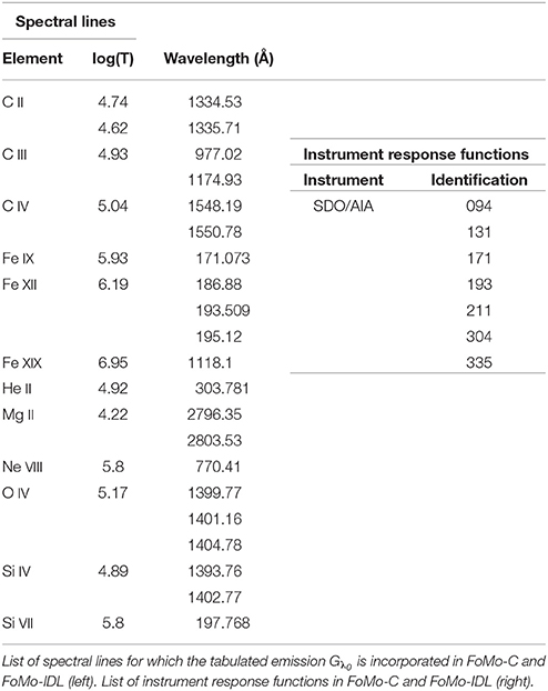
Table 1. List of tabulated emission in FoMo.

Some included line emission (such as He II, Mg II) is often observed to be optically thick. The users of the code need to ensure that the considered model (and its expected emission) is in the optically thin regime for these spectral lines, and the assumption of ionization equilibrium is not too stringent for the modeled environment.

We compute the full-width half-maximum of the spectral line λ_w (or width of Gaussian σ_w) from the temperature by

$\begin{array}{cc}\begin{array}{l}{\lambda }_{\text{w}}=2\sqrt{2\ln 2}\frac{v_{\text{th}}}{c}{\lambda }_0=2\sqrt{2\ln 2}\sqrt{\frac{kT}{{\mu }_{{\lambda }_0}{m}_{\text{p}}}}\frac{{\lambda }_0}{c},\\ \text{equivalent to taking }{\sigma }_{\text{w}}=\frac{v_{\text{th}}}{c}\frac{{\lambda }_0}{\sqrt{2}},\end{array}& (5)\end{array}$

where k is the Boltzmann constant, c is the speed of light, m_p is the mass of a proton, ${\mu }_{{\lambda }_0}$ is the atomic weight (in proton masses) of the emitting element and $v_{th}=\sqrt{\frac{2kT}{{\mu }_{{\lambda }_0}{m}_p}}$ is the thermal velocity. This is done at each voxel in FOMO-C, but only for each histogram bin in FOMO-IDL (see Section 2.3).

Thus, in this first step of the computation, the physical variables n_e, T are converted to $\widetilde{ϵ},{\lambda }_w$.

In the second step, the integration along the LOS is performed. At each voxel, the emissivity, spectral line width and velocity $\widetilde{ϵ},{\lambda }_w,\overrightarrow{v}$ are interpolated from its nearest neighbor in the (x, y, z) grid. Then the wavelength dependence of the monochromatic emissivity is calculated by taking a Gaussian shaped spectral line with the correct thermal line width (Equation 5) and the local Doppler shift.

$\begin{array}{cc}\begin{array}{l}ϵ(\lambda ,x\prime ,y\prime ,z\prime )=\frac{2\sqrt{2\ln 2}}{\sqrt{2\pi }{\lambda }_{\text{w}}}\widetilde{ϵ}(x\prime ,y\prime ,z\prime )\\ \exp \left(-\frac{4\ln 2}{{\lambda }_{\text{w}}^2}{\left(\lambda -{\lambda }_0\left(1-\overrightarrow{z^{\prime }}·\overrightarrow{v}/c\right)\right)}^2\right)\end{array}& (6)\end{array}$

$\begin{array}{cc}\begin{array}{l}=\frac{1}{{\sigma }_{\text{w}}\sqrt{2\pi }}\widetilde{ϵ}(x\prime ,y\prime ,z\prime )\\ \exp \left(-\frac{1}{2{\sigma }_{\text{w}}^2}{\left(\lambda -{\lambda }_0\left(1-\overrightarrow{z^{\prime }}·\overrightarrow{v}/c\right)\right)}^2\right)\end{array}& (7)\end{array}$

The local Doppler shift is calculated by projecting the local velocity $\overrightarrow{v}(x,y,z)$ onto a unit vector $\overrightarrow{z^{\prime }}$ along the LOS, given by

$\begin{array}{cc}\overrightarrow{z^{\prime }}=\left(\begin{array}{c}\sin b\cos l\\ -\sin b\sin l\\ \cos b\end{array}\right),& (8)\end{array}$

as can be readily derived from Equation (2). The velocity projection is done in each grid point, and then the value is interpolated to the forward modeling grid.

After summation with Equation (3), the specific intensity $I(\lambda ,x_i^{\prime },y_j^{\prime })$ is returned as a result of the second step in the code. This specific intensity can then be fitted with a Gaussian in order to obtain intensity, Doppler shift and line width. An example of this is shown in Figure 2.

FIGURE 2

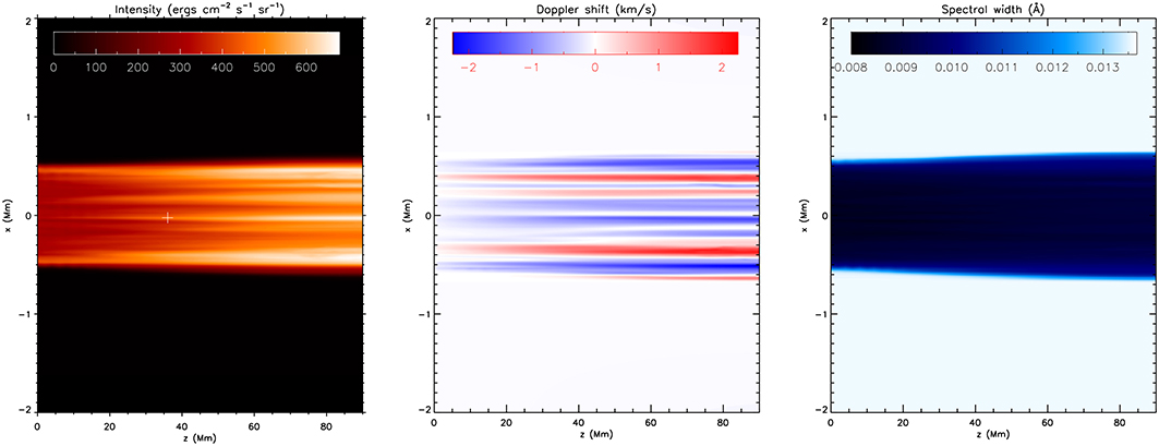
Figure 2. The typical data products from FoMo. The left panel shows the intensity, the middle panel the Doppler shift, and the right panel the line width. This rendering has been performed for the data used for the code validation in Section 2.6. The white “+” shows the position for the spectral line comparison in Figure 3.

For the calculation of emission in the imaging telescopes of SDO/AIA, we have computed instrument response functions κ_α(n_e, T) for bandpass α on a grid of densities n_e and temperatures T. For this we have used the AIA temperature response functions (obtained with aia_get_resp.pro, Boerner et al., 2012) and the contribution function G(λ, n_e, T) with the CHIANTI isothermal.pro routine (and also includes the continuum emission), following the procedure detailed in Del Zanna et al. (2011). The instrument response is then computed by

$\begin{array}{ll}{\kappa }_{\alpha }(n_e,T)={\displaystyle {\int }_{{\lambda }_{\alpha }}}G({\lambda }_{\alpha },n_e,T)R_{\alpha }({\lambda }_{\alpha })d{\lambda }_{\alpha },& (9)\end{array}$

where R_α is the wavelength-dependent response function of bandpass α, and where the wavelength integration is done over all spectral lines with wavelengths contained in the bandpass (the wavelength range is roughly centered on the dominant spectral line and has a width largely covering the FWHM given by the response function). The available instrument responses are listed in Table 1, and have been computed with both coronal and photospheric abundances.

The instrument response in the image plane of the forward model is then obtained through integrating κ_α over the LOS. Thus, the equivalent for Equation (3) for the imaging telescope is

$\begin{array}{ll}I(x_i^{\prime },y_j^{\prime })={\displaystyle \sum _k}{\kappa }_{\alpha }(x_i^{\prime },y_j^{\prime },z_k^{\prime })\Delta l,& (10)\end{array}$

in which the emissivity was replaced by the instrument response function.

The above features are common in at least FOMO-C and FOMO-IDL. In the following subsection, we will outline the specific methods used for applying the above derivation, and which optimizations have been implemented. FOMO-GS is rather different than the above procedure, since it calculates the gyrosynchrotron emission with 1D radiative transfer. It is described separately in Section 2.4.

2.2. FoMo-C v3.2

The FOMO-C code is written as shared object library, against which the user can link the code for the specific problem at hand. In the library an object FoMoObject is defined. It has several members defined:

• push_back_datapoint({x,y,z},{rho,T,vx,vy,vz}): This adds data points of the simulation to the FoMoObject.

• setresolution(nx,ny,nz,nlambda,lambdawidth): This sets the resolution of the rendering. The resolution should more or less match the resolution of the simulation.

• render(l,b): The member performing the actual rendering of the data cube, for angle l and b. The result will be written out to hard disk, for post-processing and analysis.

For more information on the members of the FoMoObject and example for the practical usage, please consult the FOMO wikipage at https://wiki.esat.kuleuven.be/FoMo/, or the documentation provided through doxygen in the source files of the code.

Interpolations in FOMO-C are performed with the CGAL library (The CGAL Project, 2015). This happens on two occasions in the code:

1. The first usage of the CGAL library occurs for the interpolation of G_λ0 [for using in Equation (4)] on the simulation grid (x, y, z) in the conversion from n_e, T to $\widetilde{ϵ}$. First the data is read in from the tabulated CHIANTI file [as a function $\widetilde{ϵ}(n_e,T)$], then a 2D triangulation is constructed of this function. Then, at each simulation point, the pair of (n_e, T) is located in the triangulation, and a linear interpolation between neighboring points is performed.

2. The second interpolation in the CGAL library is for the interpolation of the voxels into the 3D grid of the original simulation. A 3D triangulation is constructed for the grid of the simulation (using the parallel triangulation algorithm of CGAL, based on Intel's Thread Building Blocks). Thus, FOMO-C does not rely on a regular grid, and allows for the use of general grids in the simulation (including adaptive mesh refinement, and even unstructured grids). Then, each voxel is located within the 3D triangulation, and the emissivity of the nearest grid point is used as the interpolated value.

The integration along the LOS is parallelized through OpenMP tasks. Each pixel in the imaging plane is independent from other pixels, and thus constitutes a task. In the task, the processor walks along the LOS, gradually adding the (wavelength-dependent) emission to obtain the intensity in that respective pixel.

The main attraction of FOMO-C is that (1) it is built in a modular fashion, and adding of new rendering algorithms is easy, (2) it allows for having irregular grids (such as adaptive mesh refinement, or unstructured grids), (3) it is parallelized with OpenMP and Intel's Thread Building Blocks, (4) it is written and built in C++ with the GNU autotools and should thus work on a variety of systems.

The current version of FOMO-C (v3.2) contains documentation written in doxygen. Moreover, examples are provided on how to read in data and render it, including examples on the processing of HDF5 output from the FLASH code (Fryxell et al., 2000; Lee et al., 2009). Routines are also provided in order to import the FOMO-C output into IDL, where the output can be post-processed (e.g., Gaussian fitting of the spectral lines and visualization).

2.3. FoMo-IDL

FOMO-IDL has been written taking into account the numerical limitations encountered when using IDL, namely, limits on memory management, CPU speed and parallelization, all of which can make the computations significantly slower than in C++. Nevertheless, the implementations performed in the programming of the IDL version make the computations highly efficient and comparable (to some extent) to the C++ counterpart.

As mentioned in Section 2.1 the main idea behind our forward modeling is to convert the physical variables n_e, T in the numerical model to the observables $\widetilde{ϵ},{\lambda }_w$. For dealing with this conversion in an efficient manner in IDL we construct histograms of the velocity and emissivity and work with the resulting bins as groups of pixels instead of individual pixels. The constructed bins are then representations sampling the entire velocity - emissivity space. Doppler shifts and thermal width calculations are therefore applied to the groups of pixels within single bins “simultaneously” instead of pixel by pixel. Let us explain this binning procedure in more detail.

With the help of IDL's histogram function we first generate bins of the velocity space from the numerical box with a given velocity width (set by default to 0.5 km s⁻¹). Let the set of velocity bins be {_{Vi}i = 1, …, n}. The group of pixels within a bin V_i forms a set of emissivities ϵ(V_i), given by Equation (4). We then generate a second histogram, now of emissivities, for each set {ϵ(_{Vi)}i = 1, …, n}, each leading to a binning of the emissivities corresponding to a velocity v_i of the bin V_i. Let the group of emissivity bins linked to the velocity bin V_i be {_{ϵVi}j = 1, m}. Now, consider a bin ${ϵ}_{V_{ij}}$ of this second set of bins. We calculate the average temperature $T_{i,j}^{av}\equiv \overline{T({ϵ}_{{V_i}_j})}$ of the pixels within this bin. The average line width $\overline{{\lambda }_{w,T_{i,j}^{av}}}$ for this bin will then be given by Equation (5), replacing the temperature by this average temperature in the bin. The emissivity for all pixels within this bin is then set to the corresponding emissivity bin value ${ϵ}_{V_{ij}}$. A Gaussian function is then constructed for all pixels within this emissivity bin linked to the velocity bin V_i, having a total emissivity ${ϵ}_{V_{ij}}$, Doppler shifted by a velocity v_i, and with a FWHM $\overline{{\lambda }_{w,T_{i,j}^{av}}}$.

FOMO-IDL requires the numerical box to have uniform grids (although it will be extended to non-uniform grids in the future). Based on given numerical grids new grids are constructed for the voxels. The resolution in the new grids is set based on the original numerical resolution and the LOS, aiming at making the forward modeling as precise as possible. For instance, assuming that the LOS is in the (x, y) plane and that the resolution elements of the original grids are dx and dy, then the resolution step of pixels along the LOS is given by $min\left\{dy,\sqrt{({(dxcos(\theta ))}^2+{(dysin(\theta ))}^2)}\right\}$ for dx < dy and $min\left\{dx,\sqrt{({(dxcos(\theta ))}^2+{(dysin(\theta ))}^2)}\right\}$ for dy < dx (and is set equal to dx when dx = dy). Here θ is the angle in Figure 1 and the plane of the image corresponds to the (x, y) plane.

Interpolations in FOMO-IDL, as in FOMO-C, are linear and occur twice per run. The first time is for calculating the emissivity values (Equation 4) corresponding to the physical variables n_e, T in the numerical box from the look-up table of the contribution function. The second time is for the integration along the LOS in the new (uniform) grid, where, before summing, the set of Doppler shifted emissivity pixels calculated from the binning step is interpolated into the new grid along the LOS.

More details about FOMO-IDL, especially on the practical use, can be found in the online wiki of the FOMO project at https://wiki.esat.kuleuven.be/FoMo/.

2.4. FoMo-GS

FOMO-GS is an alternative version of the FOMO code in which the radio emission is computed, instead of the EUV emission (as in FOMO-C and FOMO-IDL). For EUV emission, the local density, temperature and velocity is the required information for the computation of the emission. However, for radio emission entirely different quantities are important. A first approximation for the gyrosynchrotron emission for coronal plasmas is given by Dulk and Marsh (1982). In their formulae, it is apparent that rather the magnitude and direction of the magnetic field, the number density of non-thermal particles, and the power law index of the particle distribution are important parameters for the gyrosynchrotron emission.

Thus, prior to running FOMO-GS, it is essential for the user to choose a distribution of non-thermal particles in the simulation domain. One possibility is to take the number density proportional to the total number of electrons in each simulation cell (as was done in Reznikova et al., 2014, 2015; Kuznetsov et al., 2015, although computing the density with energetic tracer particles may be more accurate). Moreover, the user needs to make a choice on the power law of non-thermal particles (which may differ from point to point in the simulation). Finally, a pitch-angle distribution for the non-thermal electrons needs to be fixed.

For the projection along the LOS, FOMO-GS follows the implementation of FOMO-IDL, using an angle l and b to rotate the simulation data cube (following Equation 2). The angle θ of the magnetic field with the LOS is computed from the simulation by

$\begin{array}{ll}cos\theta =\frac{\overrightarrow{z^{\prime }}·\overrightarrow{B}}{B},& (11)\end{array}$

where B is the magnitude of the magnetic field and the unit vector $\overrightarrow{z^{\prime }}$ along the LOS was defined in Equation (8). Then, the necessary information along the LOS is extracted by doing a nearest-neighbor interpolation of the LOS voxels into the original simulation grid.

Subsequently, the physical quantities on the LOS voxels are fed into the fast gyrosynchrotron code by Fleishman and Kuznetsov (2010). This code computes for each voxel the emissivity and absorption coefficient. It is based on the formulae given in Ramaty (1969), but implements several optimizations to speed up the computation time drastically. Then, the fast gyrosynchrotron code performs a 1D radiative transfer calculation along the LOS (see Equation 25 in Ramaty, 1969). As a result, the intensity in left- and right-polarized radio waves is obtained in each observational pixel, which allows for the computation of the intensity and polarization.

Once again, for the practical usage of FOMO-GS we refer to the wikipage of the FOMO project at https://wiki.esat.kuleuven.be/FoMo/.

2.5. Data Handling

Often the simulation data are very large. It is thus not trivial to fit all the simulation data into the computer memory, let alone the triangulation and forward model. Therefore, a clever choice of a subset of the simulation is often necessary for all three flavors of FOMO.

Alternatively, it may be possible to split the simulation in several 2D slices or 3D subsets (that contain the LOS rays), and to perform the rendering on those. Afterwards the partial artificial simulations may be rejoined. The user can write a program to do this in an automated fashion.

Such a splitting approach may also lead to further parallelization over multiple computers (e.g., with MPI), since rendering all subsets of the simulation data is independent from the other subsets and is thus massively parallel, both in computational power and memory.

2.6. Validation

For performing the code validation and performance analysis, we have taken a snapshot from simulations similar to the one in Antolin et al. (2014). In the simulation, an overdense coronal loop was simulated subjected to an initial transverse velocity. The loop starts to oscillate, and generates turbulence-like Kelvin-Helmholtz vortices at the edge. The simulation is performed for a quarter of the loop (given the symmetry of the transverse mode) with a numerical resolution of 512 × 256 × 50 points (with the smallest number of points along the magnetic field, z in Figure 2). The datacube that is fed into the forward modeling is 512 × 512 × 50, and has now also the data mirrored with respect to the mid-plane of the loop. For more details, the reader is referred to Antolin et al. (2014).

For the validation, we render the simulation at snapshot 251 in the Fe XII 193.509 Å spectral line, both with FOMO-C and FOMO-IDL. The resolution for both renderings is chosen as 724 × 50 × 100 (x′xy′xλ), and with 724 points along the LOS direction. The simulation is viewed with an angle of 45° with respect to the direction of the initial velocity perturbation. We choose a quasi-random position $(x_s^{\prime },y_s^{\prime })$ in the resulting data-cube, within the loop (i.e., where the emission is higher), indicated with a white “+” in Figure 2. In the left panel of Figure 3, we show the specific intensity $I(\lambda ,x_s^{\prime },y_s^{\prime })$ at this position, for both FOMO-C (with plusses) and FOMO-IDL (with diamonds). It is clear that the results from both codes are very close to each other.

FIGURE 3

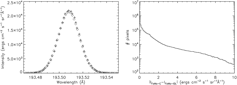
Figure 3. The left panel shows the specific intensity as a function of the wavelength, for a pixel in the center of the numerical domain. The plusses show the results from FOMO-C, while the diamonds show the results from FOMO-IDL. The right panel displays a histogram of the differences of specific intensity |I_FoMo-C − I_FoMo-IDL| between the results of FOMO-C and FOMO-IDL. The vertical axis shows the number of pixels with the deviation indicated on the horizontal axis (in ergs cm⁻² s⁻¹ sr⁻¹ Å⁻¹).

To quantify the discrepancy between the two codes better, we have displayed a histogram of the difference between the specific intensity in both codes (|I_FoMo-C − I_FoMo-IDL|) in the right panel of Figure 3. Here as well, the majority of the simulation point lie within 10 ergs cm⁻² s⁻¹ sr⁻¹ Å⁻¹ from each other, compared to a maximum specific intensity of 3 × 104 ergs cm⁻² s⁻¹ sr⁻¹ Å⁻¹.

2.7. Performance

We have compared the performance of the FOMO-IDL and FOMO-C codes using the same rendering as described in Section 2.6. The performance tests were done on a machine with two Intel Xeon E5-2630 v3 CPUs, each with eight cores (and thus 16 threads) running at 2.40 GHz. The machine has 128 GB memory. The results of the performance test are shown in Table 2.

TABLE 2

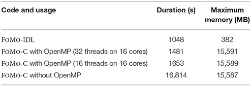
Table 2. Performance of the FoMo-C and FoMo-IDL code.

FOMO-C generally uses a lot of memory (as also shown in the table). This is mainly because of the memory-intensive computation of the triangulation by CGAL. It is clear from the table that FOMO-IDL outperforms FOMO-C. This is no surprise, because the FOMO-IDL code has been optimized for the forward modeling of regularly gridded data. Moreover, when a favorable angle is chosen along an axis of the simulation (0 or 90°), the computation time of FOMO-IDL is more than halved.

This also indicates in which direction FOMO-C could improve in future releases.

One of the advantages of FOMO-C is that it allows for easy parallelization via OpenMP. In Table 2, we have studied the computation times for FOMO-C when running with 1, 16, or 32 threads on a 16 core machine. Going from the non-parallel run to 16 threads, the code is sped up by roughly a factor 10. The non-perfect speed-up is mainly because the construction of the CGAL triangulation is not happening in parallel and the read-in and write-out times of the large data files. Adding more threads does not benefit strongly the efficiency of the computation.

In principle, it is possible to parallelize the code using MPI [chopping up the “observation” plane in roughly equal parts, and doing parallel interpolation of the emissivity $\widetilde{ϵ}$ in Equation (7)], but we have not tested this in practice.

3. Conclusions

In this article, we have given an overview of the techniques used in the FOMO code. FOMO is a numerical code for the forward modeling of emission from coronal plasmas. There are three versions of FOMO. The purpose of FOMO-C and FOMO-IDL is equivalent, and they compute the EUV emission from optically thin coronal plasmas by direct integration of the emissivity along the LOS. To this end, they both use CHIANTI emissivity tables. They both have the option to compute the emission in imaging telescopes (in particular SDO/AIA) and spectrometers (such as Hinode/EIS). FOMO-C has more features than FOMO-IDL: it also has parallelism and can perform forward modeling for non-regular grids (adaptive mesh or unstructured), although the usage of FOMO-IDL will be extended to non-uniform grids as well.

The third part of FOMO is the FOMO-GS code. FOMO-GS computes gyrosynchrotron emission from coronal plasmas. It uses the fast gyrosynchrotron codes (Fleishman and Kuznetsov, 2010) as backend to perform the 1D radiative transfer along the LOS. It thus also computes the gyrosynchrotron emission from optically thick plasmas.

FOMO was developed with the aim of performing forward modeling of coronal wave models. It has been previously used for the modeling of sausage waves (Antolin and Van Doorsselaere, 2013; Reznikova et al., 2014, 2015; Kuznetsov et al., 2015), kink waves (Antolin et al., 2014, 2015), and slow waves (De Moortel et al., 2015; Yuan et al., 2015). However, the code has a much wider applicability.

Author Contributions

TVD initiated the development of FOMO through his Odysseus grant and is the main developer for FOMO-C. PA is the main developer of FOMO-IDL. DY is a major contributor of FOMO-C. VR has written the FOMO-GS code. NM has developed the FLASH example for FOMO-C. TVD has written the first draft of the current paper, and received input from all co-authors.

Funding

Odysseus funding (FWO-Vlaanderen), IAP P7/08 CHARM (Belspo), GOA-2015-014 (KU Leuven), NAOJ Visiting Fellows Program. NM is a PhD student of the FWO-Vlaanderen.

Conflict of Interest Statement

The authors declare that the research was conducted in the absence of any commercial or financial relationships that could be construed as a potential conflict of interest.

Acknowledgments

TVD thanks the hospitality of PA and the National Astronomical Observatory of Japan during a visit in which part of the coding on FOMO was done. Discussion at the ISSI and ISSI-BJ also contributed in the development of the code. Numerical computations were carried out on Cray XC30 at the Center for Computational Astrophysics, National Astronomical Observatory of Japan.

References

Antolin, P., Okamoto, T. J., De Pontieu, B., Uitenbroek, H., Van Doorsselaere, T., and Yokoyama, T. (2015). Resonant absorption of transverse oscillations and associated heating in a solar prominence. II. Numerical aspects. Astrophys. J. 809:72. doi: 10.1088/0004-637X/809/1/72

CrossRef Full Text | Google Scholar

Antolin, P., and Van Doorsselaere, T. (2013). Line-of-sight geometrical and instrumental resolution effects on intensity perturbations by sausage modes. Astron. Astrophys. 555:A74. doi: 10.1051/0004-6361/201220784

CrossRef Full Text | Google Scholar

Antolin, P., Yokoyama, T., and Van Doorsselaere, T. (2014). Fine strand-like structure in the solar corona from magnetohydrodynamic transverse oscillations. Astrophys. J. Lett. 787:L22. doi: 10.1088/2041-8205/787/2/L22

CrossRef Full Text | Google Scholar

Arregui, I., Andries, J., Van Doorsselaere, T., Goossens, M., and Poedts, S. (2007). MHD seismology of coronal loops using the period and damping of quasi-mode kink oscillations. Astron. Astrophys. 463, 333–338. doi: 10.1051/0004-6361:20065863

CrossRef Full Text | Google Scholar

Aschwanden, M. J. (2011). Solar stereoscopy and tomography. Living Rev. Solar Phys. 8:5. doi: 10.12942/lrsp-2011-5

CrossRef Full Text | Google Scholar

Asensio Ramos, A., and Arregui, I. (2013). Coronal loop physical parameters from the analysis of multiple observed transverse oscillations. Astron. Astrophys. 554:A7. doi: 10.1051/0004-6361/201321428

CrossRef Full Text | Google Scholar

Boerner, P., Edwards, C., Lemen, J., Rausch, A., Schrijver, C., Shine, R., et al. (2012). Initial calibration of the Atmospheric Imaging Assembly (AIA) on the Solar Dynamics Observatory (SDO). Solar Phys. 275, 41–66. doi: 10.1007/s11207-011-9804-8

CrossRef Full Text | Google Scholar

De Moortel, I., Antolin, P., and Van Doorsselaere, T. (2015). Observational signatures of waves and flows in the solar corona. Solar Phys. 290, 399–421. doi: 10.1007/s11207-014-0610-y

CrossRef Full Text | Google Scholar

De Moortel, I., and Nakariakov, V. M. (2012). Magnetohydrodynamic waves and coronal seismology: an overview of recent results. R. Soc. Lond. Philos. Trans. A 370, 3193–3216. doi: 10.1098/rsta.2011.0640

PubMed Abstract | CrossRef Full Text | Google Scholar

Del Zanna, G., O'Dwyer, B., and Mason, H. E. (2011). SDO AIA and Hinode EIS observations of “warm” loops. A&A 535:A46. doi: 10.1051/0004-6361/201117470

CrossRef Full Text | Google Scholar

Dere, K. P., Landi, E., Mason, H. E., Monsignori Fossi, B. C., and Young, P. R. (1997). CHIANTI - an atomic database for emission lines. Astron. Astrophys. Suppl. 125, 149–173. doi: 10.1051/aas:1997368

CrossRef Full Text | Google Scholar

Dulk, G. A., and Marsh, K. A. (1982). Simplified expressions for the gyrosynchrotron radiation from mildly relativistic, nonthermal and thermal electrons. Astrophys. J. 259, 350–358. doi: 10.1086/160171

CrossRef Full Text | Google Scholar

Fang, X., Yuan, D., Van Doorsselaere, T., Keppens, R., and Xia, C. (2015). Modeling of reflective propagating slow-mode wave in a flaring loop. Astrophys. J. 813:33. doi: 10.1088/0004-637X/813/1/33

CrossRef Full Text | Google Scholar

Fleishman, G. D., and Kuznetsov, A. A. (2010). Fast gyrosynchrotron codes. Astrophys. J. 721, 1127–1141. doi: 10.1088/0004-637X/721/2/1127

CrossRef Full Text | Google Scholar

Fryxell, B., Olson, K., Ricker, P., Timmes, F. X., Zingale, M., Lamb, D. Q., et al. (2000). FLASH: an adaptive mesh hydrodynamics code for modeling astrophysical thermonuclear flashes. Astrophys. J. Suppl. 131, 273–334. doi: 10.1086/317361

CrossRef Full Text | Google Scholar

Gibson, S. E. (2015). Data-model comparison using FORWARD and CoMP. Proc. Int. Astron. Union 305, 245–250. doi: 10.1017/S1743921315004846

CrossRef Full Text | Google Scholar

Gibson, S., Kucera, T., White, S. M., Dove, J., Fan, Y., Forland, B., et al. (2016). FORWARD: A toolset for multiwavelength coronal magnetometry. Front. Astron. Space Sci. 3:8. doi: 10.3389/fspas.2016.00008

CrossRef Full Text

Goossens, M., Arregui, I., Ballester, J. L., and Wang, T. J. (2008). Analytic approximate seismology of transversely oscillating coronal loops. Astron. Astrophys. 484, 851–857. doi: 10.1051/0004-6361:200809728

CrossRef Full Text | Google Scholar

Gruszecki, M., Nakariakov, V. M., and Van Doorsselaere, T. (2012). Intensity variations associated with fast sausage modes. Astron. Astrophys. 543:A12. doi: 10.1051/0004-6361/201118168

CrossRef Full Text | Google Scholar

Krishna Prasad, S., Banerjee, D., and Van Doorsselaere, T. (2014). Frequency-dependent damping in propagating slow magneto-acoustic waves. Astrophys. J. 789:118. doi: 10.1088/0004-637X/789/2/118

CrossRef Full Text | Google Scholar

Krishna Prasad, S., Banerjee, D., Van Doorsselaere, T., and Singh, J. (2012). Omnipresent long-period intensity oscillations in open coronal structures. Astron. Astrophys. 546:A50. doi: 10.1051/0004-6361/201219885

CrossRef Full Text | Google Scholar

Kumar, P., Innes, D. E., and Inhester, B. (2013). Solar dynamics observatory/atmospheric imaging assembly observations of a reflecting longitudinal wave in a coronal loop. Astrophys. J. Lett. 779:L7. doi: 10.1088/2041-8205/779/1/L7

CrossRef Full Text | Google Scholar

Kumar, P., Nakariakov, V. M., and Cho, K.-S. (2015). X-Ray and EUV observations of simultaneous short and long period oscillations in hot coronal arcade loops. Astrophys. J. 804:4. doi: 10.1088/0004-637X/804/1/4

CrossRef Full Text | Google Scholar

Kuznetsov, A. A., Van Doorsselaere, T., and Reznikova, V. E. (2015). Simulations of gyrosynchrotron microwave emission from an oscillating 3D magnetic loop. Solar Phys. 290, 1173–1194. doi: 10.1007/s11207-015-0662-7

CrossRef Full Text | Google Scholar

Landi, E., Young, P. R., Dere, K. P., Del Zanna, G., and Mason, H. E. (2013). CHIANTI-an atomic database for emission lines. XIII. Soft X-Ray improvements and other changes. Astrophys. J. 763:86. doi: 10.1088/0004-637X/763/2/86

CrossRef Full Text | Google Scholar

Lee, D., Deane, A. E., and Federrath, C. (2009). “A new multidimensional unsplit MHD solver in FLASH3,” in Numerical Modeling of Space Plasma Flows: ASTRONUM-2008, volume 406 of Astronomical Society of the Pacific Conference Series, eds N. V. Pogorelov, E. Audit, P. Colella, and G. P. Zank (San Francisco, CA), 243.

Liu, W., and Ofman, L. (2014). Advances in observing various coronal EUV waves in the SDO era and their seismological applications (invited review). Solar Phys. 289, 3233–3277. doi: 10.1007/s11207-014-0528-4

CrossRef Full Text | Google Scholar

Mandal, S., Magyar, N., Yuan, D., Banerjee, D., and Van Doorsselaere, T. (2016). Forward modeling of propagating slow waves in coronal loops and its frequency-dependent damping. Astrophys. J. doi: 10.1088/0004-637X/789/2/118. Available online at: http://adsabs.harvard.edu/abs/2016arXiv160200787M

CrossRef Full Text

Marsh, M. S., Walsh, R. W., and Plunkett, S. (2009). Three-dimensional coronal slow modes: toward three-dimensional seismology. Astrophys. J. 697, 1674–1680. doi: 10.1088/0004-637X/697/2/1674

CrossRef Full Text | Google Scholar

Mossessian, G., and Fleishman, G. D. (2012). Modeling of gyrosynchrotron radio emission pulsations produced by magnetohydrodynamic loop oscillations in solar flares. Astrophys. J. 748:140. doi: 10.1088/0004-637X/748/2/140

CrossRef Full Text | Google Scholar

Nakariakov, V. M., and Ofman, L. (2001). Determination of the coronal magnetic field by coronal loop oscillations. Astron. Astrophys. 372, L53–L56. doi: 10.1051/0004-6361:20010607

CrossRef Full Text | Google Scholar

Nakariakov, V. M., and Verwichte, E. (2005). Coronal waves and oscillations. Living Rev. Solar Phys. 2:3. doi: 10.12942/lrsp-2005-3

CrossRef Full Text | Google Scholar

Nita, G. M., Fleishman, G. D., Kuznetsov, A. A., Kontar, E. P., and Gary, D. E. (2015). Three-dimensional radio and X-Ray modeling and data analysis software: revealing flare complexity. Astrophys. J. 799:236. doi: 10.1088/0004-637X/799/2/236

CrossRef Full Text | Google Scholar

Okamoto, T. J., Antolin, P., De Pontieu, B., Uitenbroek, H., Van Doorsselaere, T., and Yokoyama, T. (2015). Resonant absorption of transverse oscillations and associated heating in a solar prominence. I. Observational aspects. Astrophys. J. 809:71. doi: 10.1088/0004-637X/809/1/71

CrossRef Full Text | Google Scholar

Ramaty, R. (1969). Gyrosynchrotron emission and absorption in a magnetoactive plasma. Astrophys. J. 158:753. doi: 10.1086/150235

CrossRef Full Text | Google Scholar

Reznikova, V. E., Antolin, P., and Van Doorsselaere, T. (2014). Forward modeling of gyrosynchrotron intensity perturbations by sausage modes. Astrophys. J. 785:86. doi: 10.1088/0004-637X/785/2/86

CrossRef Full Text | Google Scholar

Reznikova, V. E., Van Doorsselaere, T., and Kuznetsov, A. A. (2015). Perturbations of gyrosynchrotron emission polarization from solar flares by sausage modes: forward modeling. Astron. Astrophys. 575:A47. doi: 10.1051/0004-6361/201424548

CrossRef Full Text | Google Scholar

The CGAL Project (2015). CGAL User and Reference Manual, 4.6.2 Edn. CGAL Editorial Board.

Van Doorsselaere, T., Nakariakov, V. M., and Verwichte, E. (2007). Coronal loop seismology using multiple transverse loop oscillation harmonics. Astron. Astrophys. 473, 959–966. doi: 10.1051/0004-6361:20077783

CrossRef Full Text | Google Scholar

Vasheghani Farahani, S., Hornsey, C., Van Doorsselaere, T., and Goossens, M. (2014). Frequency and damping rate of fast sausage waves. Astrophys. J. 781:92. doi: 10.1088/0004-637X/781/2/92

CrossRef Full Text | Google Scholar

Verwichte, E., Aschwanden, M. J., Van Doorsselaere, T., Foullon, C., and Nakariakov, V. M. (2009). Seismology of a large solar coronal loop from EUVI/STEREO observations of its transverse oscillation. Astrophys. J. 698:397. doi: 10.1088/0004-637X/698/1/397

CrossRef Full Text | Google Scholar

Wang, T. (2011). Standing slow-mode waves in hot coronal loops: observations, modeling, and coronal seismology. Space Sci. Rev. 158, 397–419. doi: 10.1007/s11214-010-9716-1

CrossRef Full Text | Google Scholar

Yuan, D., Van Doorsselaere, T., Banerjee, D., and Antolin, P. (2015). Forward modeling of standing slow modes in flaring coronal loops. Astrophys. J. 807:98. doi: 10.1088/0004-637X/807/1/98

CrossRef Full Text | Google Scholar