A Study of the Lunisolar Secular Resonance 2ω˙+Ω˙=0

1. Introduction

Thousands of man-made objects, abandoned during space missions or remnants of operative satellites, orbit around the Earth at different altitudes. Their size varies from larger pieces, like old satellites or rocket stages, to dust-size particles given by fragmentation of satellites or even by collision events, like the impact between Kosmos 2251 and Iridium 33 in 2009, or the destruction of Fengyun-1C in 2007.

The dynamics of space debris strongly differs according to the altitude from the Earth. To this end, one distinguishes 4 main regions as follows:

(i) the LEO (Low Earth Orbit) region spans the altitude from 0 to 2000 km; here the objects feel, in order of importance, the gravitational attraction of our planet, the dissipation due to the atmospheric drag, the Earth's oblateness effect, the attraction of Moon and Sun, and the solar radiation pressure;

(ii) the MEO (Medium Earth Orbit) region goes from 2000 to 30,000 km of altitude; the forces felt by the debris are like in LEO, except that there is no atmospheric drag;

(iii) the GEO (Geostationary orbit) region is located around the value of 42,164.17 km from the Earth's center; geostationary objects move with an orbital period equal to the rotational period of the Earth;

(iv) HEO (High Earth orbit) region, refers to the space region with altitude above the geosynchronous orbit.

In this work we are interested in a particular type of motion, which corresponds to a so-called secular resonance. In particular, we consider the orbital elements which are solutions of the relation

$\begin{array}{ll}\begin{array}{l}2\dot{\omega }+\dot{\Omega }=0 ,\hfill \end{array}\hfill & (1)\hfill \end{array}$

where ω denotes the argument of perigee of the debris and Ω its longitude of the ascending node. A relation like Equation (1), involving quantities moving on long time-scales, is called a secular resonance. By considering the variations of ω and Ω as just due to the effect of the main spherical harmonics of the geopotential, one can show that Equation (1) can be written just in terms of the inclination. As shown in Hughes (1980), there can be several secular resonances which depend on the inclination only. Among such resonances, Equation (1) represents a very interesting case, since it has been shown that it affects the dynamics of objects in the MEO region (Rossi, 2008; Radtke et al., 2015; Sanchez et al., 2015). Chaotic motions arise from the interaction and overlapping of nearby resonances (Rosengren et al., 2015a,b; Daquin et al., 2016).

In this paper we introduce three different models with increasing complexity, apt to study the resonance Equation (1). The simplest model is described by a one degree-of-freedom autonomous Hamiltonian, which is obtained by averaging over the fast angles and by neglecting the rates of variation of the lunar longitude of the ascending node. This model provides the essential features, like the location of stable equilibria with large as well as with small libration amplitude. The growth of the eccentricity can be easily explained by this integrable model. In the second model one does not average over the fast angles, but still retains the assumption that the longitude of the ascending node of the Moon is constant. Circulation and libration regions can be located, as well as the chaotic separatrix, although the dynamics is very complicated: overlapping of resonances, bifurcations and, as a consequence, the existence of equilibria at large eccentricities as well as at small eccentricities, variation of the amplitude of the resonance. The last model includes the variation of the lunar longitude of the ascending node and shows that large chaotic regions can appear, contributing to an irregular variation of the orbital elements.

2. The Model

We consider a space debris subject to the gravitational attraction of the Earth, including the oblateness potential, as well as the influence of Sun and Moon. This model is described by a Hamiltonian of the form

$\begin{array}{ll}{{H}={H}}_{Kep}{+{H}}_{Geo}{+{H}}_{Moon}{+{H}}_{Sun}\text{,}\hfill & (2)\hfill \end{array}$

which is the sum of different contributions that we are going to explain and express in terms of the Delaunay action–angle variables (L, G, H, M, ω, Ω), where the actions are defined by

$\begin{array}{ll}L=\sqrt{{\mu }_{E}a},G=L\sqrt{1-e^2},H=G\cos I,\hfill & (3)\hfill \end{array}$

with μ_E = ${G}$m_E the product of the gravitational constant ${G}$ and the Earth's mass m_E, a the semimajor axis, e the orbital eccentricity, I the inclination, while the angle variables are the mean anomaly M, the argument of perigee ω, the longitude of the ascending node Ω, which are expressed with respect to the equatorial plane.

The first term in Equation (2) represents the Keplerian part ${H}$_Kep, which can be expressed as

$\begin{array}{ll}{H}\begin{array}{l}{}_{Kep}(L)=-\frac{{\mu }_E^2}{2L^2} .\hfill \end{array}\hfill & (4)\hfill \end{array}$

The second term ${H}$_Geo describes the perturbation due to the Earth, when considering the shape of our planet. In particular, we will consider only the most important term of the expansion in spherical harmonics of the geopotential, the so-called J₂-term. Indeed, while studying the long-term dynamics of resonant orbits, the short-periodic terms that depend on the mean anomaly of the satellite (as well as the mean anomaly of the perturbing body, when dealing with Sun and Moon) can be averaged over from the disturbing function. Therefore, in the expression for ${H}$_Geo we take an average of the Hamiltonian over the mean anomaly of the space debris, which implies to consider only the most important contribution, corresponding to the J₂ gravity coefficient of the secular part (see, e.g., Celletti and Galeş, 2014, compare also with Celletti and Galeş, 2015). This leads to express ${H}$_Geo in the form:

$\begin{array}{ll}{H}\begin{array}{l}{}_{Geo}(L,G,H)=\frac{R_E^2{J}_2{\mu }_E^4}{4} \frac{1}{L^3{G}^3} (1-3\frac{H^2}{G^2}) ,\hfill \end{array}\hfill & (5)\hfill \end{array}$

where R_E is the mean equatorial radius of the Earth and $J_2=1.08263\times 10^{-3}$.

The contributions due to Moon and Sun are simplified by averaging over the fast angles, precisely the mean anomaly of the debris and the mean anomalies of the perturbers (Moon and Sun). Moreover, we truncate the potentials to second order in the ratio of semi-major axes (see Kaula, 1962; Lane, 1989; Celletti et al., 2016b for details), thus obtaining the expression for ${H}$_Sun and the (quite long) expression for ${H}$_Moon, reported in Supplementary Section (see also Cook, 1962). Adding the contributions in Equations (4), (5) as well as ${H}$_Sun and ${H}$_Moon, we obtain the Hamiltonian Equation (2).

Since the mean anomaly M is a cyclic variable, its conjugated action L (or equivalently the semi-major axis a) is constant. As a consequence, the Hamiltonian system described by Equation (2) is non-autonomous with two degrees of freedom. As it was remarked by Rosengren et al. (2015a), Daquin et al. (2016), and analytically shown in Celletti et al. (2016b), the Hamiltonian ${H}$ depends on time just through the longitude of lunar ascending node Ω_M with a rate of variation equal to ${\dot{\Omega }}_M\simeq -0.053^{°}∕day$, which implies a periodicity of Ω_M over 18.6 years. More precisely, since ${\dot{\Omega }}_S=0$, where Ω_S is the longitude of the solar ascending node, and the expansions of the lunar and solar potentials to second order in the ratio of semimajor axes are independent of the lunar and solar perigees, it follows that ${H}$ depends on time only through Ω_M.

To a first approximation we assume that the Moon orbits on an elliptic trajectory with semimajor axis equal to a_M = 384, 748 km, eccentricity e_M = 0.0549006 and inclination $I_M=5^{°}15^{\prime }$; the mass m_M of the Moon, expressed in Earth's masses, is about equal to 0.0123. The orbital elements of the Moon are referred to the ecliptic plane.

As for the Sun, we can assume that its elements are constants and, precisely, a_S = 149, 597, 871 km, eccentricity e_S = 0.01671123 and inclination $I_S=23^{°}26^{\prime }21.406^{″}$; the mass of the Sun m_S, expressed in Earth's masses, is approximately equal to 333,060.4016. The orbital elements of the Sun are expressed with respect to the equatorial plane.

The model described by Equation (2) gives all the ingredients to capture the main dynamical features of the resonant structure within the MEO region (see Rosengren et al., 2015a for a comparison between various models).

3. The Secular Resonance $2\dot{\omega }+\dot{\Omega }=0$

In this Section we are interested to the so-called (lunar and solar) secular resonances, which occur whenever one has a commensurability between the arguments of perigee and the longitudes of the nodes of the debris and the perturbers, according to the following definition.

Definition 1. A lunar gravity secular resonance occurs whenever there exists an integer vector $(k_1,k_2,k_3)\in {\mathbb{Z}}^3\backslash \left\{0\right\}$, such that

$\begin{array}{ll}\begin{array}{l}{k}_1\dot{\omega }+k_2\dot{\Omega }+k_3{\dot{\Omega }}_M=0 .\hfill \end{array}\hfill & (6)\hfill \end{array}$

We have a solar gravity secular resonance whenever there exist $(k_1,k_2,k_3)\in {\mathbb{Z}}^3\backslash \left\{0\right\}$, such that

$\begin{array}{ll}\begin{array}{l}{k}_1\dot{\omega }+k_2\dot{\Omega }+k_3{\dot{\Omega }}_S=0 .\hfill \end{array}\hfill & (7)\hfill \end{array}$

We can assume that the rate of variation ${\dot{\Omega }}_S$ is zero, while for the Moon we will build different models according to which the rate ${\dot{\Omega }}_M$ is zero or it is rather equal to ${\dot{\Omega }}_M\simeq -0.053^{°}∕day$.

As for the debris, we can approximate $\dot{\omega }$, $\dot{\Omega }$ by considering only the effect of J₂ (Hughes, 1980):

$\begin{array}{ll}\begin{array}{c}\dot{\omega }\simeq 4.98{\left(\frac{R_E}{a}\right)}^{\frac{7}{2}} {(1-e^2)}^{-2} (5{\cos }^{2}I-1){ }^{°}/day ,\hfill \\ \dot{\Omega }\simeq -9.97{\left(\frac{R_E}{a}\right)}^{\frac{7}{2}} {(1-e^2)}^{-2} \cos I{ }^{°}/day .\hfill \end{array}\hfill & (8)\hfill \end{array}$

Inserting Equation (8) in Equation (6) or Equation (7), we get an expression which involves the orbital elements a, e, I, thus providing the location of the secular resonance.

A remarkable fact (see Hughes, 1980) is that some resonances depend only on the inclination and are independent on a, e. Precisely, following Hughes (1980) we can identify the following classes of lunisolar secular resonances depending only on inclination (see Figure 1):

(i) $\dot{\omega }=0$, which occurs at the critical inclinations I = 63.4°, I = 116.6°;

(ii) $\dot{\Omega }=0$, which corresponds to polar orbits;

(iii) $\alpha \dot{\omega }+\beta \dot{\Omega }=0$ for some nonzero α, β ∈ ℤ.

FIGURE 1

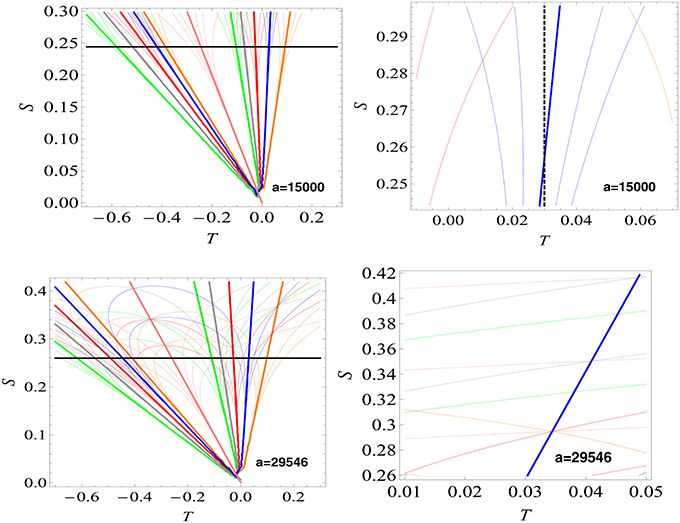
Figure 1. The web structure of resonances in the space of the actions for a = 15, 000 km (upper panels) and a = 29, 546 km (bottom panels). The thick curves represent the location of the following exact resonances (the multiplet component having s = 0): $\dot{\Omega }=0$ (pink color, I = 90°), $\dot{\omega }-\dot{\Omega }=0$ (green color, I = 73.2°, I = 133.6°), $2\dot{\omega }-\dot{\Omega }=0$ (gray color, I = 69.0°), I = 123.9°, $\dot{\omega }=0$ (red color, I = 63.4°, I = 116.6°), $2\dot{\omega }+\dot{\Omega }=0$ (blue color, I = 56.1°, I = 111°) and $\dot{\omega }+\dot{\Omega }=0$ (orange color, I = 46.4°, I = 106.9°). The thin curves give the position of the resonances $(2-2p)\dot{\omega }+m\dot{\Omega }+s{\dot{\Omega }}_k=0$ with p, m = 0, 1, 2 and s = −2, −1, 1, 2. The vertical black dashed line (top right panel) corresponds to the values of T used in computing the Figure 6. Left panels are obtained for S ∈ [0, S_max], whereas in the right plots S varies from S_min to S_max, as explained in the text.

In this work we are interested to a specific resonance of type (iii) and precisely to the resonance

$\begin{array}{ll}\begin{array}{l}2\dot{\omega }+\dot{\Omega }=0 .\hfill \end{array}\hfill & (9)\hfill \end{array}$

Using Equations (8) and (9), one can write this resonances as

$2\dot{\omega }+\dot{\Omega }={\left(\frac{R_E}{a}\right)}^{\frac{7}{2}} {(1-e^2)}^{-2} \left[9.96(5{\cos }^{2}I-1)-9.97\cos I\right]=0 ,$

whose solutions are I = 56.1° and I = 111.0°, independently of the values of semimajor axis and eccentricity.

In writing Equation (9) we have implicitly assumed that ${\dot{\Omega }}_M=0$ (as we mentioned, the other rates ${\dot{\omega }}_M$, ${\dot{\omega }}_S$, ${\dot{\Omega }}_S$ can be assumed to be equal to zero). However, Ω_M varies periodically and some arguments of ${H}$_Moon could depend also on Ω_M. Therefore, besides $2\dot{\omega }+\Omega =0$, one also has the commensurability relations

$\begin{array}{ll}\begin{array}{l}2\dot{\omega }+\Omega +s{\dot{\Omega }}_M=0 , s=-2,-1,1,2 .\hfill \end{array}\hfill & (10)\hfill \end{array}$

This means that the secular resonance splits into a multiplet of resonances. This splitting phenomenon is responsible for the existence of a very complex web-like background of resonances in the phase space, which leads to a chaotic variation of the orbital elements. An analytical estimate of the location of the resonance corresponding to each component of the multiplet, as a function of eccentricity and inclination, can be obtained by using Equation (8) (see, for example, Figure 2 in Ely and Howell, 1997 or Rosengren et al., 2015a).

To describe properly the dynamics, it is convenient to use resonant variables, which are introduced through the symplectic transformation (G, H, ω, Ω) → (S, T, σ, η) defined by

$\begin{array}{ll}\begin{array}{l}\sigma =2\omega +\Omega ,S=\frac{G}{2},\\ \eta =\Omega ,T=H-\frac{G}{2}.\end{array}\hfill & (11)\hfill \end{array}$

Since we expressed the Hamiltonian in Delaunay variables, we represent in Figure 1 the web structure of resonances in the space of the actions T–S introduced in Equation (11). To avoid confusions that might arise when we speak about a specific resonance, we will use the terminology exact resonance when we refer to the component of the multiplet characterized by s = 0 in Equation (10), while the expression whole resonance means that we refer to all components of the multiplet.

We underline that the units of length and time are normalized so that the geostationary distance is unity (it amounts to 42, 164.17 km) and that the period of the Earth's rotation is equal to 2π. As a consequence, from Kepler's third law it follows that μ_E = 1. Therefore, unless the units are explicitly specified, the action variables L, S and T are expressed in the above units.

Figure 1 shows the structure of resonances for a = 15, 000 km (top panels) and a = 29, 546 km (bottom panels). The colored curves provide the location of the resonances, while the vertical black dashed line in the top-right panel is drawn to provide the value of T used in computing the FLI plot for a = 15, 000 km (see Figure 6). In order to show graphical evidence of the splitting phenomenon, Figure 1, left panels, provide the resonant structure for S ∈ [0, S_max], where $S_{max}=\frac{\sqrt{{\mu }_{E}a}}{2}$. These plots contain also the horizontal black line S = S_min, where S_min is computed from the condition that the distance of the perigee cannot be smaller than the radius of the Earth, that is

$S_{min}=\frac{1}{2}\sqrt{\frac{(2a-R_E){\mu }_E{R}_E}{a}} .$

Therefore, the interval of interest is [S_min, S_max]. The right panels of Figure 1 magnify the regions associated to the orbits that do not collide with the Earth (at least for a small interval of time). Figure 1 shows the complicated interplay of the web of resonances, with multiple crossings of lines, which correspond to overlapping of resonances, possibly providing a mechanism for the onset of chaos (Chirikov, 1979; Daquin et al., 2016).

4. A Comparison of Different Models

In order to understand the complicated dynamics of the whole resonance $2\dot{\omega }+\dot{\Omega }=0$, we shall simplify further the model described in the previous Section. In fact, we consider three different models, based on the Hamiltonian function introduced in Equation (2):

a) The one degree-of-freedom autonomous Hamiltonian, obtained by averaging ${H}$ in Equation (2) over the fast angle η and by neglecting the rates of variation of Ω_M. Indeed, we use the constant value ${\Omega }_M=125.045^{°}$, valid at epoch J2000.

b) The two degrees-of-freedom autonomous Hamiltonian, derived under the assumption that the rate of variation of Ω_M is negligible. Again, we use the constant value ${\Omega }_M=125.045^{°}$, valid at epoch J2000.

c) The non-autonomous Hamiltonian ${H}$, defined by Equation (2).

The following sections describe in detail the results which are obtained using models a–c.

4.1. Results for Model A

The results obtained integrating model a, the simplest model as possible, are shown in Figure 2, which provides the phase space portraits for a = 15, 000 km and a = 29, 546 km. In order to show more clearly the structure of the phase space, in all figures we represent the resonant angle σ = 2ω+Ω on intervals longer than 360°.

FIGURE 2

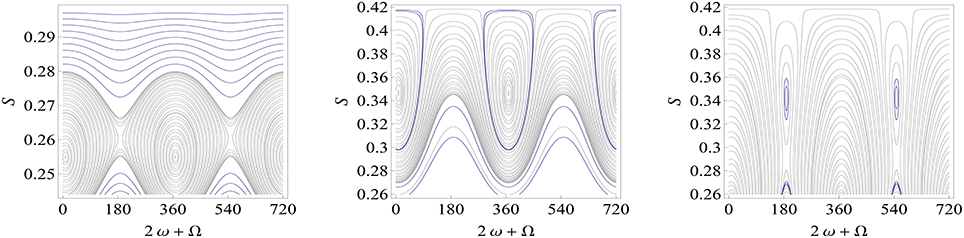
Figure 2. Phase space portraits for a = 15, 000 km and T = 0.03 (left panel), a = 29, 546 km and T = 0.05 (middle panel), a = 29, 546 km and T = 0.03 (right panel).

Figure 2 shows that for sufficiently small values of the semimajor axis (left panel) the phase space has a pendulum-like structure, while for larger values of the semimajor axis (middle and right panels) the pendulum-like model is no longer valid. In fact, for a = 29, 546 km, a bifurcation phenomenon appears, showing that there are some cases when a specific resonance cannot be modeled by a pendulum type system, but one should use a more complex model, referred in the literature as the extended fundamental model (see Breiter, 2001; Celletti et al., 2016a for details).

Comparing the right panel of Figure 2, obtained for T = 0.03, with the middle panel of the same Figure 2, computed for T = 0.05, we notice the appearance of a new elliptic point, located at σ = 180°. Besides this phenomenon, it is important to note that the main stable point, which is located at σ = 360° (or 0°), changes its position in the action space as a function of T. For instance, for T = 0.05, this point is located at S = 0.3407 [or at e = 0.581, as it follows from Equations (3), (11)], while for T = 0.03, it is positioned at S = 0.26 (or e = 0.784). Figure 2 middle plot reveals the fact that none of the orbits located inside the libration region of the elliptic point will collide with the Earth, while in Figure 2 right plot, all orbits located inside the libration region associated with the main elliptic point are colliding orbits.

The integrable model a gives a clear explanation for the growth of the eccentricity of the satellites and space debris revolving around the Earth on orbits having an inclination about equal to 56°. In fact, the growth of the eccentricity is mainly due to the dynamical feature of the resonance. Inside the libration region, the resonant angle σ = 2ω + Ω and its conjugated action S vary periodically. Since, the eccentricity e is related to S through the relation $e=\sqrt{1-\frac{4S^2}{T^2}}$, then it follows naturally that the eccentricity varies in time.

4.2. Results for Model B

To analyze model b we use the Fast Lyapunov Indicators (hereafter, FLI), which are defined as the largest Lyapunov characteristic exponents at a fixed time (compare with Celletti and Galeş, 2014). We provide the definition of FLI in Supplementary Materials. Their values provide a numerical indication of the stable (low values) and chaotic (high values) behavior of the dynamical system as the initial conditions or some internal parameters are varied.

We shall focus on a = 29, 546 km, because for a = 15, 000 km the phase plane σ–S, even in the case of the full model c, is similar to a pendulum, as it is shown in Figure 6.

The results for model b are given in Figures 3–5. Thus, given a = 29, 546 km and a value for T, we compute a grid of 100 × 100 points of the σ–S plane, where the resonant angle ranges in the interval [0°, 360°] (also here we use a larger interval just to show better the structure of the phase space), while S spans the interval [S_min, S_max]. However, instead of displaying S on the vertical axis, in each plot we show the eccentricity values (on the left) and the inclination values (on the right), computed by using the relations (3) and (11) for given values of T. In all plots that represent the FLI values, we use the ranges corresponding to those used in the right panels of Figure 1. The relation among S, T, e and I is trivial; for instance, the value e = 0.784 from the left panel of Figure 3 corresponds to the value S = 0.26 from the top right panel of Figure 1, while the value I = 52.02° from the same left panel of Figure 3 corresponds to the values S = 0.26 and T = 0.06.

FIGURE 3

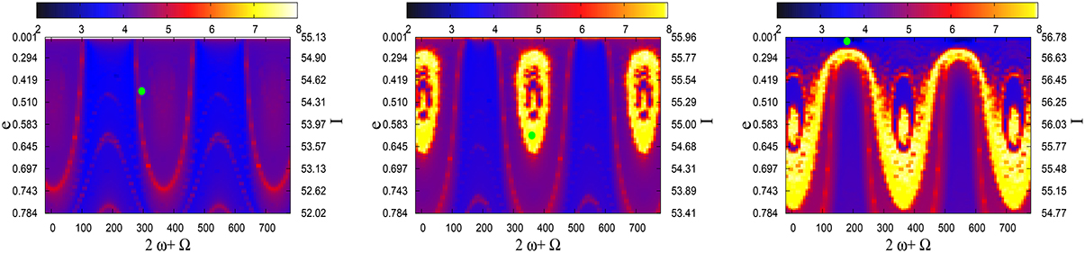
Figure 3. FLIs for the model b, for a = 29, 546 km, Ω = 180° and: T = 0.06 (left), T = 0.05 (middle), T = 0.04 (right). Each plot contains one green circle. These circles represent the orbits analyzed in Figure 4.

Although the initial conditions are set such that the initial orbits have the perigee larger than R_E, since we are interested in understanding the mean dynamical features of the $2\dot{\omega }+\dot{\Omega }=0$ resonance, during the total time of integration, we neglect the Earth's dimensions. Namely, we propagate each orbit up to 465 years (equal to 25 × 18.6 years), even if at some intermediate time the perigee distance becomes smaller than the radius of the Earth.

As we mentioned in Section 4.1, for large values of the semimajor axis in model a, the phase space is much more complicated than the one associated to the pendulum model. The complexity increases when we consider the two degrees-of-freedom autonomous Hamiltonian of model b. In fact, the manifolds defined by ${H}$(S, T, σ, η) = const. have dimension three in the four dimensional phase space ℝ² × ${\mathbb{T}}^2$. This makes difficult the visualization of phase portraits or even the interpretation of the FLI plots. However, we can draw some conclusions from Figures 3, 5, obtained by projecting the phase space on the plane (σ, S), for fixed values of T and η.

In fact, we underline three aspects concerning the global dynamics, which are revealed by the model b, namely: the amplitude of resonance depends on the values of both canonical variables T and η. For some values of the canonical variables, the resonances $2\dot{\omega }+\dot{\Omega }=0$ and $\dot{\omega }=0$ overlap; the bifurcation phenomenon, revealed by the model a, is observable both in this case but also in the case of the full model c.

The plots shown in Figure 3 are obtained for η = 180° and different values of its conjugated action T, while Figure 5 shows some results obtained for the same value of T and various values of η. Moreover, in order to have a clear idea about the patterns shown in these plots, in Figure 4 we represent the evolution of the eccentricity, inclination and the resonant angle for three distinct orbits. Thus, the orbit depicted by the top plots of Figure 4 (the green circle in the left panel of Figure 3) is located inside the libration region; the eccentricity and resonant angle vary periodically. In the middle panels of Figure 4 (see also the green circle of the middle panel of Figure 3) we consider an orbit located inside the region where the resonances $2\dot{\omega }+\dot{\Omega }=0$ and $\dot{\omega }=0$ are so close that there is a non negligible interaction; we integrate the orbit over a longer time (930 years), even if it is a colliding orbit just to show the strong interaction of the above mentioned resonances. Over a period of 350 years the orbit is located inside the libration region of the resonance $2\dot{\omega }+\dot{\Omega }=0$, then, after an interval of time, it escapes from that resonance and it is rather captured into the critical inclination resonance. Finally, the bottom plots of Figure 4 correspond also to a resonant orbit (the green circle of the right panel of Figure 4): they do not belong to the main resonant libration region, but rather to the resonant small region which appears as a result of the bifurcation phenomenon, already described by the model a.

FIGURE 4

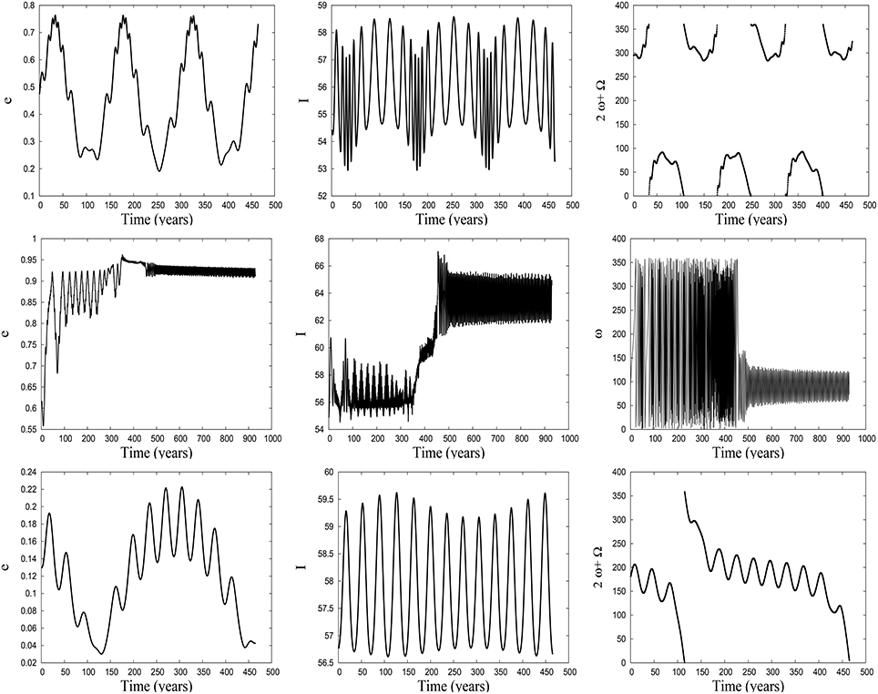
Figure 4. Integration of the orbits having the initial conditions Ω = 180° and: σ = 295°, T = 0.06, S = 0.37 (or e = 0.467, I = 54.47°) (top plots); σ = 360°, T = 0.05, S = 0.33 (or e = 0.615, I = 54.85°) (middle plots); σ = 180°, T = 0.04, S = 0.415 (or e = 0.13, I = 56.76°) (bottom plots).

In conclusion, the global dynamics revealed by the model b is very complex: overlapping of resonances (the yellow regions¹ in Figures 3, 5), bifurcations and, as a consequence, the existence of equilibria at large eccentricities as well as at small eccentricities, variation of the amplitude of the resonance as a function of T and η (compare, for instance, the small libration zone of the left plot of Figure 5 with the large libration regions from the middle and right plots again of Figure 5).

FIGURE 5

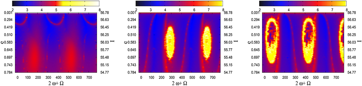
Figure 5. FLIs for the model b, for a = 29, 546 km, T = 0.04 and: Ω = 0° (left); Ω = 90° (middle); Ω = 270° (right).

4.3. Results for Model C

We finally consider the dynamics associated to the more complete model c, which is described by the non-autonomous Hamiltonian ${H}$ introduced in Equation (2) The results are presented in Figures 6–8. As we already remarked above, for a = 15, 000 km, the phase plane σ–S is very similar to the one described by model a, compare Figure 6 with the left panel of Figure 2. However, for large a, the dynamics is much more complex. Roughly speaking, on the global dynamical background described by model b, and which does not change significantly in a vicinity of several km from the nominal distance of a = 29, 546 km, one should superimpose the exact resonances shown in different colors in the right bottom panel of Figure 1. These resonances are due to the variation of the lunar node, as noted by Ely and Howell (1997), Rosengren et al. (2015a), and their location depends on the value of the semimajor axis.

FIGURE 6

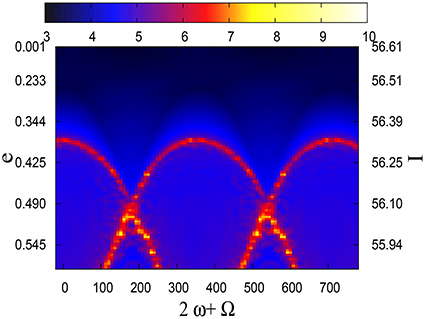
Figure 6. FLIs for the model c, for a = 15, 000 km, Ω = 180° and T = 0.03.

As a consequence, since the resonance $2\dot{\omega }+\dot{\Omega }=0$ is crossed by multiple exact resonances, having different widths (see Daquin et al., 2016), the orbital elements vary chaotically. One gets large regions filled by chaotic motions, marked by larger yellow-red values of the FLI. In contrast with the model b, here the FLI values vary on a longer scale, from 2 to 14. Figure 7 shows the results for T = 0.04 and for Ω = 0° (left), Ω = 90° (middle) and Ω = 180° (right). Comparing these plots with the corresponding ones obtained for model b, we remark that, besides the large yellow-red regions obtained as effect of the overlapping of resonances (either the superposition of the exact resonances shown in the right bottom panel of Figure 1 with the exact resonance $2\dot{\omega }+\dot{\Omega }=0$, or with the critical inclination resonance $\dot{\omega }=0$), some blue regions are noticeable, which account for the libration regions associated to the equilibrium points. For instance, in the left plot of Figure 7, we have a stable equilibrium point at about σ = 360° and e = 0.294 with a libration island (blue color) small in width (compare also with the left plot of Figure 5). Numerical tests show that an initial condition inside this region remains there, even if the variations of e and σ are not regular. The red-yellow regions visible for eccentricities larger than 0.5 are due to the interaction of the exact resonances depicted in Figure 1, bottom right plot, with the critical inclination resonance.

FIGURE 7

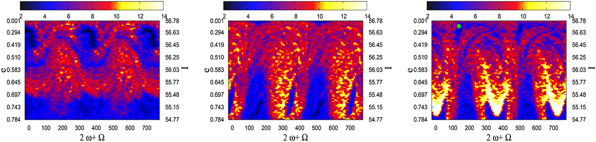
Figure 7. FLIs for the model c, for a = 29, 546 km T = 0.04 and: Ω = 0° (left); Ω = 90° (middle); Ω = 180° (right). The green circle in the right plot represents an orbit analyzed in Figure 8.

In both the middle and right panels of Figure 7, we notice two important blue (libration) regions: one at small eccentricities (the orbit marked with a green circle in the right panel of Figure 7 and analyzed in Figure 8 is within this region) and one at large eccentricities (at about σ = 360° and e = 0.784 in the right panel of Figure 7). These regions show that the bifurcation phenomenon described by the model a is still valid for the more complete model c.

FIGURE 8

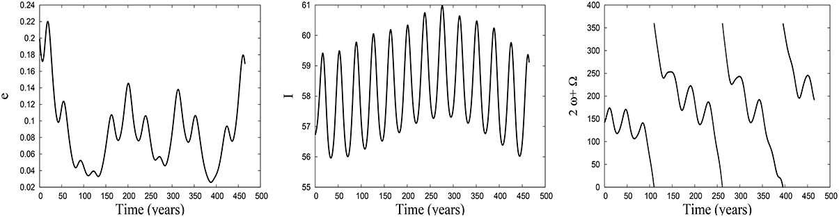
Figure 8. Integration of the orbit having the initial conditions T = 0.04, Ω = 180°, σ = 142° and S = 0.41 (or e = 0.201, I = 56.71°).

As a final remark, one should clarify what is happening inside the yellow-red region, for example in the middle panel of Figure 7. The answer is the following: usually one obtains an irregular growth in eccentricity. The growth is due, in essence, to the resonance $2\dot{\omega }+\dot{\Omega }=0$ (as the models a and b infer) and the irregular (chaotic) behavior is obtained as an effect of the overlapping of the resonance $2\dot{\omega }+\dot{\Omega }=0$ with the resonances shown in Figure 1. We made several other experiments and found that colliding orbits can occur as a byproduct of the eccentricity growth due to the interaction with the resonance $2\dot{\omega }+\dot{\Omega }=0$: the increase of the eccentricity leads to have a distance at perigee less than the Earth's radius. On the other hand, initial data in a chaotic region can undergo the effect of the interaction between different resonance, but without leading to collisions.

5. Conclusions

Lunisolar resonances might contribute to shape the dynamics of small bodies around the Earth (Breiter, 2001; Rosengren et al., 2015a; Daquin et al., 2016). Among such resonances, that corresponding to $2\dot{\omega }+\dot{\Omega }=0$ is responsible for the growth in eccentricity. To explain this phenomenon, we compare three different models with increasing complexity, obtained averaging over fast angles (model a), or just by neglecting the rate of variation of Ω_M (model b), or rather including the variation of Ω_M (model c). A comparison among these models provide us with the ingredients which lead to chaos and which provide an increase of the eccentricity.

By comparing the results of models a–c, we infer that the dynamics around the stable equilibria at large values of the eccentricity is well represented by all models. On the contrary, for small values of the eccentricity the effect of the variation of the lunar longitude of the node plays a relevant role and, even if it occurs on long time scales, cannot be neglected for an accurate description of the dynamics.

Finally, it is worth noticing that the growth in eccentricity provoked by the resonance $2\dot{\omega }+\dot{\Omega }=0$ can be used as an effective strategy to move space debris into non-operative or graveyard orbits.

Author Contributions

The paper has been written by both authors in equal parts.

Conflict of Interest Statement

The authors declare that the research was conducted in the absence of any commercial or financial relationships that could be construed as a potential conflict of interest.

Acknowledgments

AC was partially supported by the European Grant MC-ITN Stardust, PRIN-MIUR 2010JJ4KPA_009 and GNFM/INdAM; CG was supported by a grant of the Romanian National Authority for Scientific Research and Innovation, CNCS - UEFISCDI, project number PN-II-RU-TE-2014-4-0320 and by GNFM/INdAM.

Supplementary Material

The Supplementary Material for this article can be found online at: https://www.frontiersin.org/article/10.3389/fspas.2016.00011

Footnotes

1. ^For the critical inclination resonance, the stable equilibrium points are located at ω = 90° and ω = 270°.

References

Breiter, S. (2001). Lunisolar resonances revisited. Celest. Mech. Dyn. Astr. 81, 81–91. doi: 10.1007/978-94-017-1327-6_10

CrossRef Full Text | Google Scholar

Celletti, A., and Galeş, C. (2014). On the dynamics of space debris: 1:1 and 2:1 resonances. J. Nonlin. Sci. 24, 1231–1262. doi: 10.1023/A:1013363221377

CrossRef Full Text | Google Scholar

Celletti, A., and Galeş, C. (2015). A study of the main resonances outside the geostationary ring. Adv. Space Res. 56, 388–405. doi: 10.1016/j.asr.2015.02.012

CrossRef Full Text | Google Scholar

Celletti, A., Galeş, C., and Pucacco, G. (2016a). Bifurcation of lunisolar secular resonances for space debris orbits. arXiv: 1512.02178.

Celletti, A., Galeş, C., Pucacco, G., and Rosengren, A. (2016b). Analytical development of the lunisolar disturbing function and the critical inclination secular resonance. arXiv: 1511.03567.

Chirikov, B. V. (1979). A universal instability of many-dimensional oscillator systems. Phys. Rep. 52, 263–379. doi: 10.1016/0370-1573(79)90023-1

CrossRef Full Text | Google Scholar

Cook, G. E. (1962). Luni-solar perturbations of the orbit of an Earth satellite. Geophys. J. 6, 271–291. doi: 10.1111/j.1365-246X.1962.tb00351.x

CrossRef Full Text

Daquin, J., Rosengren, A. J., Alessi, E. M., Deleflie, F., Valsecchi, G. B., Rossi, A., et al. (2016). The dynamical structure of the MEO region: long-term stability, chaos, and transport. Celest. Mech. Dyn. Astr. 124, 335–366. doi: 10.1007/s10569-015-9665-9

CrossRef Full Text | Google Scholar

Ely, T. A., and Howell, K. C. (1997). Dynamics of artificial satellite orbits with tesseral resonances including the effects of luni–solar perturbations. Dyn. Stabil. Syst. 12, 243–269. doi: 10.1080/02681119708806247

CrossRef Full Text | Google Scholar

Froeschlé, C., Lega, E., and Gonczi, R. (1997). Fast Lyapunov indicators. Application to asteroidal motion. Celest. Mech. Dyn. Astr. 67, 41–62. doi: 10.1023/A:1008276418601

CrossRef Full Text | Google Scholar

Hughes, S. (1980). Earth satellite orbits with resonant lunisolar perturbations. I. Resonances dependent only on inclination. Proc. R. Soc. Lond. A 372, 243–264. doi: 10.1098/rspa.1980.0111

CrossRef Full Text | Google Scholar

Kaula, W. M. (1962). Development of the lunar and solar disturbing functions for a close satellite. Astron. J. 67, 300–303. doi: 10.1086/108729

CrossRef Full Text | Google Scholar

Lane, M. T. (1989). On analytic modeling of lunar perturbations of artificial satellites of the Earth. Celest. Mech. Dyn. Astr. 46, 287–305. doi: 10.1007/BF00051484

CrossRef Full Text | Google Scholar

Radtke, J., Dominguez-Gonzalez, R., Flegel, S. K., Sanchez-Ortiz, N., and Merz, K. (2015). Impact of eccentricity build-up and graveyard disposal Strategies on MEO navigation constellations. Adv. Space Res. 56, 2626–2644. doi: 10.1016/j.asr.2015.10.015

CrossRef Full Text | Google Scholar

Rosengren, A. J., Alessi, E. M., Rossi, A., and Valsecchi, G. B. (2015a). Chaos in navigation satellite orbits caused by the perturbed motion of the Moon. Mon. Not. R. Astron. Soc. 449, 3522–3526. doi: 10.1093/mnras/stv534

CrossRef Full Text | Google Scholar

Rosengren, A. J., Daquin, J., Alessi, E. M., Deleflie, F., Rossi, A., Valsecchi, G. B., et al. (2015b). Galileo disposal strategy: stability, chaos and predictability. arXiv:1512:05822v1

Rossi, A. (2008). Resonant dynamics of Medium Earth Orbits: space debris issues. Celest. Mech. Dyn. Astr. 100, 267–286. doi: 10.1007/s10569-008-9121-1

CrossRef Full Text | Google Scholar

Sanchez, D. M., Yokoyama, T., and de Almeida Prado, A. F. B. (2015). Study of some strategies for disposal of the GNSS satellites. Math. Probl. Eng. 2015:382340. doi: 10.1155/2015/382340

CrossRef Full Text | Google Scholar