Prospects for Measuring Planetary Spin and Frame-Dragging in Spacecraft Timing Signals

1. Introduction

General relativity (GR) describes gravitation as a consequence of a curved four dimensional spacetime (Iorio, 2015; Debono and Smoot, 2016). In most astrophysical systems, however, dynamics are dominated by Newtonian physics and GR only provides very small perturbations. Near a mass M, the relativistic perturbations on an orbiting or passing body depend mostly on the pericenter distance, which we call p, in units of the gravitational radius GM/c². Newtonian effects are of order O(p^−1/2). The largest relativistic perturbation is time dilation, and is of O(p⁻¹). Space curvature, referring to space-space terms in the metric tensor, enters dynamics at O(p^−3/2). At O(p⁻²) mixed space-time metric terms enter the dynamics; these correspond to frame-dragging effects, in which a spinning mass drags spacetime in its vicinity and thereby affects the orbit and orientation of objects in its gravitational field. Gravitational radiation corresponds to dynamical effects of O(p⁻³). In post-Newtonian notation, X PN (e.g., 1 PN, 2 PN, …) corresponds to O(p^−X−1/2). In the Solar System, p is very large in gravitational terms: ~10⁸ or more. In close binary systems p can be much less. In binary pulsars the combination of comparatively low p ~ 10⁵ with the long-term stability of pulsar timing enables the measurement of relativistic effects down to gravitational radiation (Taylor, 1994; Kramer et al., 2006).

All the same effects are, in principle, present for artificial Earth satellites, but since p ~ 10⁹, they are much weaker. Nonetheless, until now the frame-dragging effect of the Earth's spin has been detected in two different ways: (1) the LAGEOS and LARES satellites used laser ranging to measure orbital perturbations from frame-dragging (Ciufolini and Pavlis, 2004; Ciufolini et al., 2016) (some aspects are still controversial Iorio et al., 2011; Renzetti, 2013, 2015; Iorio, 2017); (2) Gravity Probe B measured the effects of frame-dragging on the orientation of onboard gyroscopes (Everitt et al., 2011). GPS satellites are well known to be sensitive to time dilation (Ashby, 2003) and upcoming missions will put even more precise clocks in orbit. In the Atomic Clock Ensemble in Space (ACES) mission (Cacciapuoti and Salomon, 2011), two atomic clocks will be brought to the ISS in order to perform such experiments. However, the ISS is not the optimal place to probe GR and a dedicated satellite on a highly eccentric orbit would be desirable. Its proximity to Earth and high velocity at pericenter would boost relativistic effects and therefore improve the measurements. Several such satellites equipped with an onboard atomic clock and a microwave or optical link on very eccentric orbits, such as STE-QUEST, have been discussed and studied (Altschul et al., 2015). Such missions would not only be very interesting to probe gravity but also have a plethora of applications, e.g., in geophysics (Bondarescu et al., 2012, 2015).

Missions like Juno and Cassini present new possibilities for measuring relativistic effects around the giant planets in our Solar System. The basic idea goes back to the early days of general relativity, when Lense and Thirring (Lense and Thirring, 1918) showed that the orbital plane of a satellite precesses about the spin axis of the planet—that is what we now call frame-dragging— and identified the expected precession of Amalthea's orbit by 1′53″ per century as the most interesting case. Recent work has drawn attention to the corresponding precession in the case of Juno (Iorio, 2010, 2013; Helled et al., 2011) and other systems (Iorio, 2005, 2011, 2012).

The classical Lense-Thirring precession is an orbit-averaged effect. This comes with the problem that the very small precession due to relativity is masked by much larger non-relativistic precession, making it very hard to identify the relativistic contribution. For example, most of Mercury's observed precession is due to Newtonian planetary perturbations, the relativistic contribution being only about 7% of the total (Park et al., 2017). It is better to have something with a specific time dependence that can be filtered out.

Here, we extend the work of Angélil et al. for terrestrial satellites (Angélil et al., 2014) and the Galactic center (Kannan and Saha, 2009; Preto and Saha, 2009; Angélil and Saha, 2010; Angélil and Saha, 2011, 2014; Angélil et al., 2010; Zhang and Iorio, 2017) and apply it to other planets in the Solar System. Since the orbits are dominated by Newtonian physics, and relativity only contributes very small perturbations, their investigation is numerically challenging. In earlier work (Angélil et al., 2014) the orbits were therefore simulated with smaller semi-major axes compared to the real orbit and then, by knowing how the individual effects scale, the redshift curves were obtained by correctly scaling up. Here, we use an arbitrary precision code instead.

We look at an idealized model where a spacecraft sends electromagnetic signals to a ground station. Comparing the relativistic 4-momentum of the emitted photon to that of the one received at the station allows determining a redshift z (see Equation 3). Equivalently, one can consider an orbiting clock which sends out signals corresponding to the ticks of the clock (Angélil and Saha, 2010; Angélil et al., 2014). Then, the redshift arises when two photons emitted by the spacecraft at an interval of proper time Δτ travel through curved spacetime hitting the observer with a difference in the arrival time Δt = Δτ(1+z). In both cases, a one-way signal transfer is considered. Typically, satellite communication systems allow two-way signal transfer. For a comparison of distant ground clocks like done with ACES, this leads to a first order cancellation of the position errors of the clocks (Duchayne et al., 2009).

To estimate the relativistic effects, we solve for the trajectory of

1. the satellite in a curved spacetime, and

2. the photons (or propagating ticks from the frequency standard) as they propagate to the receiving station

in a given gravitational field. Both the satellite and the photons follow geodesics of the metric and can be obtained by integrating the relativistic Hamiltonian, expanded in velocity orders. The redshift depends on both the classical Doppler shift as well as a number of relativistic effects. Both trajectories are generated numerically via a simulation code that handles multiple scales through variable precision. The effects are modulated by the varying gravitational field.

The paper proceeds as follows: Section 2 describes the approximations we make for the spacetime outside a planet. It presents the Hamiltonian system that is being solved numerically with the higher order relativistic effects, and their respective scalings with orbital size. We then compute the magnitude of the spin parameter, of Schwarzschild precession and frame-dragging effects for the planets in our Solar System, and report them relative to the effects around Earth for orbits of similar proportionality. Sections 4.1 and 4.2 apply this formalism to the Juno and Cassini Missions. Section 4.3 discusses the Galileo 5 and 6 satellites and other proposed Earth-bound missions. In particular, it discusses the importance of eccentricity in detecting relativistic effects.

Conclusions and potential future directions are presented in Section 5.

2. General Relativistic Effects

Calculating relativistic effects fundamentally involves two things: the metric and the geodesic equations. The well-known epigram by J.A. Wheeler states Spacetime tells matter how to move, matter tells spacetime how to curve. The metric is known explicitly in terms of the masses, including mass multipoles, and spin rates. The geodesic equation, in general, requires a numerical solution. However, in special or approximate cases analytical solutions also exist (Klioner and Kopeikin, 1992; Ashby and Bertotti, 2010; D'Orazio and Saha, 2010; Hees et al., 2014; Crosta et al., 2015).

We wish to understand how different terms in the metric, in particular the spin part, affect the observable redshift signal. To do this, we will numerically integrate the geodesic equations with different metric terms turned on and off and compare the resulting redshift signal curves.

In Section 2.1 we briefly introduce the Hamiltonian formalism and the formula for calculating the redshift. This is followed by Section 2.2, which discusses the expansion of both the orbital as well as the signal Hamiltonian. In Section 2.3 we discuss the spin parameter and in Section 2.4 we discuss the cumulative changes of the Keplerian elements due to orbital relativistic effects. Finally, in Section 2.5 we investigate how the sizes of the relativistic signals scale for the different planets in the Solar System.

2.1. Basic Formulation

We work with the geodesic equations in four dimensions, in Hamiltonian form. The independent variable is not time, but the affine parameter, which is just the proper time in arbitrary units. Although the formalism seems complex, it actually tends to lead to simpler equations (Angélil and Saha, 2010; Angélil et al., 2014) than other formulations.

For any spacetime metric, the geodesic equations may be expressed in Hamiltonian form as

$\begin{array}{ll}\frac{d{x}^{\mu }}{d\lambda }=\frac{\partial H}{\partial p_{\mu }}\frac{d{p}_{\mu }}{d\lambda }=-\frac{\partial H}{\partial x^{\mu }}& (1)\end{array}$

where

$\begin{array}{ll}H=\frac{1}{2}{g}^{\mu \nu }(x^{\alpha })p_{\mu }{p}_{\nu }& (2)\end{array}$

with x^μ = (t, rⁱ) being the four-dimensional coordinates, p_μ = (p_t, p_i) being the canonical momenta, and λ being the affine parameter.

The satellite at position $\overrightarrow{r}=(r^i)$ orbiting with 4-velocity $u_{\mathrm{\text{emit}}}^{\mu }$ emits a photon with 4-momentum $p_{\mu }^{\mathrm{\text{emit}}}$ which arrives at an observer (having velocity $u_{\mathrm{\text{obs}}}^{\nu }$) with momentum $p_{\nu }^{\mathrm{\text{obs}}}$. The redshift is then given by

$\begin{array}{ll}z=\frac{p_{\mu }^{\text{emit}}{u}_{\text{emit}}^{\mu }}{p_{\nu }^{\text{obs}}{u}_{\text{obs}}^{\nu }}-1.& (3)\end{array}$

For a distant observer at rest, the redshift for orbital effects reduces to

$\begin{array}{ll}z=\frac{1}{c}{u}_{\text{emit}}^t-\frac{1}{c}{u}_{\text{emit}}^{\text{LOS}}-1,& (4)\end{array}$

where $u_{\mathrm{\text{emit}}}^{\mathrm{\text{LOS}}}$ is the satellite's velocity along the line of sight.

2.2. The Expanded Hamiltonian

In this subsection we use geometrized units. That is, $\overrightarrow{r}$ is measured in units of GM/c² where M is the planetary mass, while t is measured in units of GM/c³. The momentum is dimensionless. Since the orbits considered are close to Keplerian, the order-of-magnitude relations

$\begin{array}{ll}|\overrightarrow{p}|~\frac{\upsilon }{c},r~{\left(\frac{\upsilon }{c}\right)}^{-2}& (5)\end{array}$

will hold, where v is the orbital speed. The time-momentum p_t is constant and its value only affects internal units of a calculation. It is convenient to set p_t = −1.

As usual in post-Newtonian celestial mechanics, we order contributions in powers of υ/c. These correspond to different physical effects. Moreover, the ordering in powers of υ/c is different for the spacecraft orbit and the light signals. Accordingly, we consider two Hamiltonians, as follows.

$\begin{array}{l}{H}^{\text{orbit}}=H^{\text{equiv-prin}}+H^{\text{Schwarzschild}}+H^{\text{spin}}\\ H^{\text{signal}}=H^{\text{Minkowski}}+H^{\text{Shapiro}}& (6)\end{array}$

Since there is only one spacetime, H^orbit and H^signal are just different approximations to the same underlying Hamiltonian.

The orbit of the satellite is dominated by

$\begin{array}{ll}{H}^{\text{equiv-prin}}=-\frac{p_t^2}{2}+\left(-p_t^{2}U(\overrightarrow{r})+\frac{{\overrightarrow{p}}^2}{2}\right)& (7)\end{array}$

where $U(\overrightarrow{r})$ is minus the Newtonian gravitational potential, to leading order 1/r but also including multipole moments J_n as well as the tidal potential due to the Sun and other planets. The first term on the right is of order unity, while the bracketed part is of order v²/c². This Hamiltonian leads to a Newtonian orbit and redshift contribution of order v/c, together with a time dilation effect of order v²/c². Gravitational time dilation is a basic consequence of the geometric description of spacetime, i.e., the principle of equivalence. Indeed, Equation (7) is the simplest Hamiltonian consistent with the equivalence principle that gives the correct Newtonian limit. Moving clocks tick slower than stationary ones. So do clocks in a gravitational field. For an orbiting clock, both effects are equal to leading order. The ground station will have its own time dilation too, of course, and the difference is what matters. Time dilation causes the localization of a satellite to be off by kilometers, which has already been taken into account by the early phases of GPS. While this relativistic effect is well established, the Galileo satellites will measure it to unprecedented precision.

Since higher order relativistic effects cause small changes in the redshift, they can be studied perturbatively. We investigate each effect individually by adding it to H^equiv-prin, and computing the cumulative redshift. The redshift perturbation is obtained by subtracting the redshift when the effect is artificially turned off.

The next contribution to H^orbit is

$\begin{array}{ll}{H}^{\text{Schwarzschild}}=-\frac{p_t^2}{r^2}-\frac{{\overrightarrow{p}}^2}{r}& (8)\end{array}$

which introduces the effect of space curvature in the Schwarzschild spacetime. It is easy to verify from Equation (5) that the Hamiltonian terms are of order sυ⁴/c⁴, and they contribute to redshift at order sυ³/c³, where s is the spin parameter. Note that the s is larger for planets (~10²−10³) than for more compact systems like black holes (s ~ 1) and thus the spin terms are significantly larger than what one would expect from just looking at velocity order.

The leading-order frame-dragging effect arises when adding the term

$\begin{array}{ll}{H}^{\text{spin}}=-\frac{2p_t}{r^3}\overrightarrow{p}·(\overrightarrow{s}\times \overrightarrow{r}).& (9)\end{array}$

This term is of order sυ⁵/c⁵ and contributes a redshift effect of order sυ⁴/c⁴. Frame-dragging is due to the rotation of the central mass, which spins with $\overrightarrow{s}$, and depends linearly on the spin parameter $s=\left|\overrightarrow{s}\right|$. At next higher order, the dominant term is a spin-squared term, i.e., it is proportional to s² (Angélil et al., 2014). This effect has never been measured before. But since s is quite large for planets (see Table 1), probing this effect should be within the scope of future satellite missions.

TABLE 1

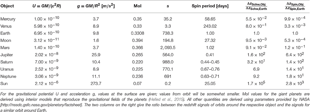
Table 1. Gravitational and spin parameters for the planets and the Moon.

The leading multipole contribution comes from J₂ in the Newtonian Hamiltonian Equation (7) and scales as 1/r³. Therefore, it has a different r-dependence as the relativistic effects discussed here. The relativistic effect with the same r-scaling would be the spin-squared effect.

The main contribution to the redshift comes from the velocity along the line of sight. Therefore, in order to measure a certain relativistic effect, it is desirable to have an orbit-observer-configuration where the relativistic effect has a significant contribution to the line of sight velocity. For first order spin, the leading contribution is given by

$\begin{array}{ll}\Delta z_{\text{spin}}=-\frac{2}{r^2}\overrightarrow{s}·(\widehat{r}\times \widehat{b}),& (10)\end{array}$

where $\widehat{b}$ is the unit vector pointing from the satellite toward the observer. Interestingly, the spin related redshift contribution has no explicit dependence on the satellite's velocity.

The signal photons travel to leading order on a straight line. The leading relativistic effect, leading to a slight bending, is Shapiro delay. This part is best analyzed after transforming to a Solar System frame. The signal Hamiltonian is given by the sum of

$\begin{array}{ll}{H}^{\text{Minkowski}}=-\frac{p_t^2}{2}+\frac{{\overrightarrow{p}}^2}{2}& (11)\end{array}$

and

$\begin{array}{ll}{H}^{\text{Shapiro}}=-U(\overrightarrow{p})\left(p_t^2+{\overrightarrow{p}}^2\right).& (12)\end{array}$

At the next order of expansion, further Shapiro-like terms as well as spin terms appear. However, they are expected to be too small to be measured. The effect of frame-dragging on light signals was calculated, e.g., by Kopeikin (1997) and Wex and Kopeikin (1999).

2.3. The Spin Parameter

The dimensionless spin parameter of a celestial body is given by

$\begin{array}{ll}s=\frac{c}{G{M}^2}{\displaystyle \int \rho }(\overrightarrow{x})\omega (\overrightarrow{x})r_{\perp }^2{d}^3\overrightarrow{x}.& (13)\end{array}$

For solid-body rotation (ω = 2π/P, where P is the spin period) the above expression reduces to

$\begin{array}{ll}s=2\pi \times \text{MoI}\times \frac{c}{gP}& (14)\end{array}$

where

$\begin{array}{ll}\text{MoI}=\frac{1}{M{R}^2}{\displaystyle \int \rho }(\overrightarrow{x})r_{\perp }^2{d}^3\overrightarrow{x}& (15)\end{array}$

is the dimensionless moment of inertia and g = GM/R² is the surface gravity, where R is the average radius of the body. For realistic density and ω profiles

$\begin{array}{ll}s~\frac{c}{gP}& (16)\end{array}$

is still a useful rough estimate. It may be convenient to remember it as the number of days needed to reach the speed of light from an acceleration of one g.

For yet another interpretation of the spin parameter, let us consider two speeds: the surface speed of a spinning planet v_s ~ R/P and the launching speed needed to send something into orbit from the surface ${\upsilon }_l^2~gR$. In terms of these speeds, the approximate formula (16) becomes

$\begin{array}{ll}s~\frac{c{v}_s}{{\upsilon }_l^2}\text{.}& (17)\end{array}$

The maximal-spinning situation v_s ≈ υ_l corresponds to a planet spinning so fast that it almost breaks up under centrifugal forces. In this limit s ~ c/υ_l. Recalling the orders in H^spin in Equation (9), we can see that that Hamiltonian term would be of order υ⁴/c⁴ and the corresponding redshift effect would be of order υ³/c³. That is, for a low-orbiting spacecraft above a maximally-spinning planet, relativistic spin effects will be comparable in size to space-curvature effects.

2.4. Keplerian Elements

A Keplerian orbit is described by the Keplerian elements a, e, Ω, I, and ω. While a and e describe the size and the eccentricity of the ellipse, the three angles describe its orientation with respect to some reference plane.

For a relativistic orbit this is not true anymore, as the relativistic effects induce deviations from Keplerian motion. In principle, however, it is still possible to determine the instantaneous Keplerian elements at each point along the orbit: These correspond to a Keplerian orbit having exactly the same velocity as the relativistic one at a given position.

It is well-known that space curvature leads to a precession of the pericenter

$\begin{array}{ll}\Delta {\omega }_{\text{Schwarzschild}}=\frac{GM}{c^2}\frac{6\pi }{a(1-e^2)}& (18)\end{array}$

for one orbit.

However, ω is not shifted evenly along the orbit, in fact, there is almost no shift during most of the orbit, but around pericenter there is a kick-like shift. Similarly, there is a precession of the pericenter due to frame-dragging (Lense and Thirring, 1918; Mashhoon et al., 1984)

$\begin{array}{ll}\Delta {\omega }_{\text{Spin}}=-s\frac{12\pi \sqrt{GM}\cos I}{{\left[a(1-e^2)\right]}^{3/2}}& (19)\end{array}$

per orbit and also there is a precession of the longitude of the ascending node

$\begin{array}{ll}\Delta {\Omega }_{\text{Spin}}=s\frac{4\pi \sqrt{GM}}{{\left[a(1-e^2)\right]}^{3/2}}& (20)\end{array}$

per orbit. Figure 1 shows the precession of the longitude of the ascending node together with the actual shift for a typical Juno orbit.

FIGURE 1

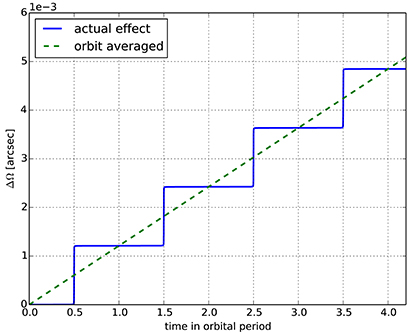
Figure 1. Change of the longitude of the ascending node Ω for a typical Juno orbit due to spin. The solid line shows the actual change of Ω, while the dashed line represents the averaged change given by Equation 20.

Measuring time-averaged precessions is not actually a useful strategy, because the slightest use of spacecraft engines changes all the Keplerian elements. But similarly to the Keplerian elements, relativistic effects affect the observed redshift in a kick-like manner at pericenter. Therefore, relativistic effects influence a single pericenter passage and when the instrument is accurate enough, they can be probed as a function of time vs. waiting for their build up over many orbits.

2.5. Scaling of Relativistic Effects

The size of the effects scale with the size of the orbit (Angélil and Saha, 2010). For Schwarzschild space curvature and first order spin, the respective scaling laws for the residual redshifts are $\Delta z^{\mathrm{\text{Schwarzschild}}}~{(r_G/r)}^{3/2}$ and $\Delta z^{\mathrm{\text{Spin}}}~s{(r_G/r)}^2$ where $r_G=GM/c^2$ is the gravitational radius. Writing distances in terms of planetary radii r = αR, we obtain

$\begin{array}{ll}\frac{\Delta z_1}{\Delta z_2}={\left(\frac{s_1}{s_2}\right)}^m{\left(\frac{r_G^1}{r_G^2}\frac{r_2}{r_1}\right)}^n={\left(\frac{s_1}{s_2}\right)}^m{\left(\frac{U_1}{U_2}\frac{{\alpha }_2}{{\alpha }_1}\right)}^n,& (21)\end{array}$

where $U_i=G{M}_i/(R_i{c}^2)$ is the gravitational potential at the surface of planet i and m = 0, 1 and n = 3/2, 2 for Schwarzschild curvature and first order spin effect, respectively. For similar orbits around different planets, i.e., α₁ = α₂ with the same eccentricity and identical Keplerian angles, this reduces to $\Delta z_1/\Delta z_2={(s_1/s_2)}^m{(U_1/U_2)}^n$. Thus, the higher the compactness M/R of a planet, the higher the relativistic effect. For frame-dragging effects, the spin parameter has also to be taken into account.

Using the expression above, we can compare the sizes of relativistic effects of orbits around the planets, the Moon and the Sun to terrestrial orbits. The ratio between the signals for similar orbits is given in Table 1.

3. Planetary Parameters

The planetary parameters relevant for calculating relativistic effects are summarized in Table 1. The Moon and the Sun are also included for comparison.

The values of the gravitational potential U at the surface are ordered as one might expect. Jupiter with 2 × 10⁻⁸ has the highest, while for the Earth the value is 30 times smaller.

The values of the spin parameter may be surprising. Black holes must have s < 1 as is well known, but planets can have s ≫ 1. Mars has the highest s ~ 2090, while Venus has the lowest s ~ 3, but most planets have an s with a value that is typically in the hundreds. Incidentally, the Sun's spin parameter will be small: The Sun has a much larger g than any planet, and it spins differentially, roughly once a month; as a result, the Sun has a much smaller s than the Earth. The uncertainty in s depends on the uncertainties in the MoI and in the spin period.

Although neither the density profile nor internal differential rotation can be measured directly, internal structure models provide MoI values for the gas giants, and these are thought to be accurate to a few percent (Helled, 2011; Helled et al., 2011; Nettelmann et al., 2015). The Radau-Darwin approximation (Zharkov and Trubitsyn, 1980) relates the MoI to the gravitational quadrupole J₂ and the ratio of centrifugal to gravitational acceleration at the equator. In future it may become possible to measure planetary MOI from precession (Maistre et al., 2016). At present, the estimated MoI is ~0.265 for Jupiter (Helled et al., 2011) and ~0.220 for Saturn (Guillot and Gautier, 2007; Helled, 2011). Evidently, Saturn is more centrally condensed than Jupiter.

The rotation period remains somewhat uncertain for all the giant planets other than Jupiter (Helled et al., 2009, 2010, 2015). Saturn's internal rotation period is unknown to within ~10 min. It has been acknowledged that the rotation period is unknown since Cassini 's Saturn kilometric radiation (SKR) measured a rotation period of 10 h 47 m 6 s (Gurnett et al., 2007), longer by about 8 min than the radio period of 10 h 39 m 22.4 s measured by Voyager (Ingersoll and Pollard, 1982). In addition, during Cassini 's orbit around Saturn the radio period was found to be changing with time. It then became clear that SKR measurements do not represent the rotation period of Saturn's deep interior. Due to the alignment of the magnetic pole with the rotation axis, Saturn's rotation period cannot be obtained from magnetic field measurements (Sterenborg and Bloxham, 2010). Theoretical efforts to infer the rotation period (Anderson and Schubert, 2007; Read et al., 2009; Helled et al., 2015) indicate further sources of uncertainty. Saturn's rotation period is thought to be between ~10 h 32 m and ~10 h 47 m. For Uranus and Neptune, the uncertainty could be as large as 4 and 8%, respectively (Helled et al., 2010).

A further complexity arises from the fact that the giant planets could have non-body rotations (e.g., differential rotation on cylinders/spheres) and/or deep winds. However, in that case, the deviation from a mean solid-body rotation period is expected to be small. Future space missions to Uranus and/or Neptune, performing accurate measurements of their gravitational fields, could be used to determine the spin parameter of these planets.

4. Relativistic Effects for Current and Planned Missions

We now determine the effects of relativity on the redshift signal for different orbits around different planets. In Section 4.1 we consider a typical orbit of the Juno spacecraft around Jupiter, followed by a typical Cassini orbit around Saturn in Section 4.2. Finally, in Section 4.3, we discuss terrestrial orbits.

4.1. Jupiter Orbit

On July 4, 2016, the Juno mission arrived at Jupiter and started orbiting the planet. It is equipped to perform high precision measurements (operating at X-band and Ka-band) of its gravitational field. The 53-days orbits are polar with perijove being at ~1.09 Jupiter radii and apojove at ~120 Jupiter radii. Such orbits provide ideal conditions for gravitational field measurements, and allow the spacecraft to avoid most of the Jovian radiation field. After more than 4 years of measurementes and ~32 orbits around Jupiter, Juno is planned to make one last orbit and then perform the deorbiting maneuver (see e.g., Matousek, 2007).

We compute the leading-order relativistic effects on the orbit of the Juno mission. They measure the precession of the orbit due to the curvature of the spacetime and contain a part that accumulates as well as a transient part, which has never been measured. The effect that occurs due to the Schwarzschild term in the Hamiltonian produces a Mercury-like precession (solid red curve), while the other is referred to as frame-dragging due to the spin of Jupiter. Measuring the latter directly constrains the spin parameter of the planet, which is proportional to its moment of inertial and angular momentum. It thus reveals important information about the planet's internal density structure that is not necessarily identical to that contained in the gravitational moments.

The Juno orbiter has already entered a highly elliptical polar orbit around Jupiter. It is measuring deviations in the velocity of the spacecraft ~10 μm/s (τ/60 s)^−1/2. This corresponds to a sensitivity to redshift change of Δz ~ 3 × 10⁻¹⁴.

At each pericenter passage of Juno, both the instantaneous Keplerian elements and the orientation to the observer change. Therefore, in order to discuss relativistic effects on the basis of the Juno mission, we consider a typical orbit with average values a = 60 × R_Jupiter, e = 0.981, Ω = 253°, I = 93.3°, ω = 170° and observer position ${\theta }_{\mathrm{\text{obs}}}=92.9°$ (polar angle), ${\varphi }_{\mathrm{\text{obs}}}=15.0°$ (azimuthal angle). Figure 2 shows the characteristic redshift curves for the different effects for such a Juno orbit. For all science orbits, the sizes of the effects, in particular of the spin effect, are similar.

FIGURE 2

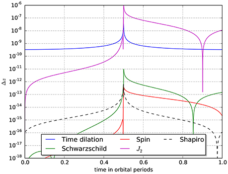
Figure 2. Higher order relativistic effects for the Juno orbiter. The plot shows the magnitude of the redshift signal due to the different relativistic effects. The parameters chosen correspond to a typical science orbit. The curves change slightly for other orbits, however, the order of magnitude of the effects is the same. Also the Newtonian effect due to J₂ is shown.

Figure 3 shows the part in the redshift due to the presence of Jupiter's spin over one orbit. After pericenter passage, the relativistic and the non-relativistic orbit are out of sync and a comparison does not make sense anymore. The lower panel of the figure zooms into the peak around pericenter, revealing that the interesting time span is of order ~1 h. This is the phase that needs to be observed in order to seek the characteristic imprint of frame-dragging in the redshift data.

FIGURE 3

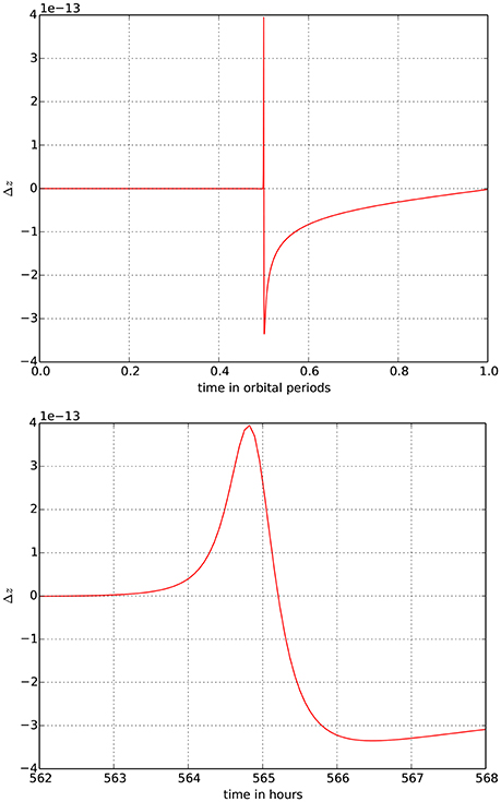
Figure 3. (Upper) contribution to the redshift from frame-dragging by Jupiter's spin, for the same orbit as in Figure 2. The signal peaks at the orbit pericenter passage. (Lower) zoom into pericenter passage.

Over any one orbit, only one component of the spin vector contributes at leading order, namely the spin component along ${\widehat{r}}_{\text{peri}}\times \widehat{b}$ (see Equation 10). To be sensitive to all components of the spin, orbits with different orientations of ${\widehat{r}}_{\text{peri}}\times \widehat{b}$ are needed. Figure 4 shows the polar and azimuthal angles of this vector for all the Juno science orbits. The orientations are varied, and hence Juno is sensitive to all three components of the spin vector.

FIGURE 4

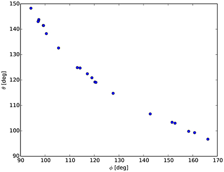
Figure 4. Orientation of the vector ${\widehat{r}}_{\text{peri}}\times \widehat{b}$ for Juno science orbits. Here $\widehat{b}$ is the line of sight to Juno, and θ, ϕ in the Figure are with respect to to Jupiter's axis. The timing signal is sensitive to the planetary spin projected along these various directions.

The frame-dragging effect will, moreover, be a pathfinder to measuring yet weaker effects. The spin terms depend on the spin profile inside the planet. Measuring the spin profile would therefore play a role in constraining planet properties and formation models. Future deep-space missions could enable tests of general relativity around other planets in the Solar System whose composition and internal structure are unknown.

4.2. Saturn Orbit

The Cassini mission is planned to finish its exploration of the Saturnian system with proximal orbits around Saturn that will provide accurate measurements of the gravitational field of the planet. The Cassini spacecraft is planned to execute 22 highly inclined (63.4°) orbits with a periapsis of ~1.02 Saturn radii (Edgington and Spilker, 2016). These proximal orbits, known as Cassini Grand Finale, operating at X-band, are also ideal for gravity measurements. They are expected to provide range rate accuracies of ~12 μm/s at 1,000 s integration times, being about four times noisier than Juno.

Both the Juno and the Cassini spacecrafts will terminate their operations by descending into the atmospheres of Jupiter and Saturn, respectively, and will disintegrate and burn up in order to fulfill the requirements of NASA's Planetary Protection Guidelines.

Cassini has a sensitivity that is about Δ z ~ 10⁻¹³. Relativistic effects peak around the pericenter with the frame-dragging effect of maximum amplitude ~10⁻¹³ and the Schwarzschild curvature term of ~10⁻¹¹. Ideally, the goal would be to resolve both the Schwarzschild and frame-dragging parts of the precession as a function of time. If they could be modeled effectively, they would less likely be drowned by Newtonian noise than a cumulative effect.

Figure 5 shows the corresponding curves for a typical Cassini orbit. For Cassini, we chose the values a = 10 × R_Saturn, e = 0.9, Ω = 175°, I = 62°, ω = 187°, ${\theta }_{\mathrm{\text{obs}}}=63.3°$ and ${\varphi }_{\mathrm{\text{obs}}}=-5°$.

FIGURE 5

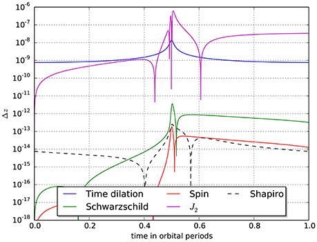
Figure 5. Higher order relativistic effects for Cassini.

4.3. Earth Orbit

Next we discuss satellites in Earth orbit. To illustrate the importance of eccentricity, Figure 6 shows the redshift curve for a typical terrestrial satellite with a low eccentricity (e = 0.1561, a = 27′977km) as for the Galileo 5 and 6 satellites and a high eccentricity (e = 0.779, a = 32′090km) orbit, while leaving all other Keplerian elements as well as the observer's position constant. However, the actual curve depends highly on the orientation of the orbit and the position of the observer and must be computed individually for each orbit-observer-configuration. Also, that the visibility of the satellite around pericenter might not be provided needs to be taken into account. For the Galileo satellites, the curve would be significantly flatter—without a clear peak around pericenter due to the low eccentricity. The only relativistic effect besides time dilation that is within the measurability range is the Schwarzschild space curvature effect. It is expected that it will improve the currently best measurement given by Gravity Probe A (Delva et al., 2015).

FIGURE 6

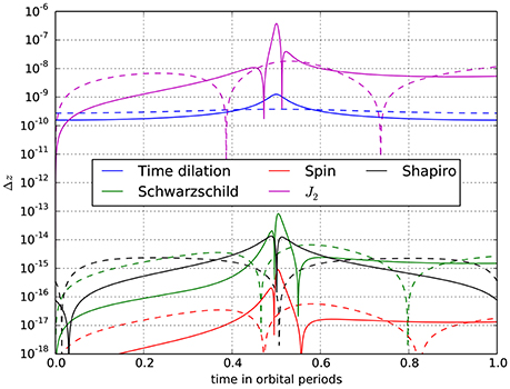
Figure 6. Redshift curves of terrestrial satellites. The dashed curves give the results for an orbit with the semi-major axis and eccentricity corresponding to the ones of the Galileo 5 and 6 satellites. The solid lines give the results for a typical satellite with high eccentricity while all the other Keplerian elements and the observer's position were left the same.

5. Conclusions

A spinning body causes spacetime to rotate around it, thus making nearby angular momentum vectors precess. This had already been considered theoretically in the early days of general relativity (Lense and Thirring, 1918). Only in recent years, however, has the effect entered the experimental realm (Ciufolini and Pavlis, 2004; Everitt et al., 2011; Ciufolini et al., 2016).

Frame-dragging is usually thought of as a steady precession. For highly eccentric orbits, however, this is far from the case. While having a minor impact along most of the orbit, frame-dragging kicks in around pericenter. This can be seen in Figure 1 which shows the change of the longitude of ascending node due to spin for some example orbits of the Juno spacecraft. An analogous situation applies to the S stars in orbit around the Galactic-center black hole (Angélil and Saha, 2014). We suggest that these pericenter-kicks could provide a distinctive signature in timing signals obtained from spacecraft tracking.

The frame-dragging contribution to the redshift of spacecraft signals is

$\begin{array}{ll}\Delta z_{\text{spin}}=-2{\left(\frac{GM}{c^{2}r}\right)}^2\overrightarrow{s}·(\widehat{r}\times \widehat{b})& (22)\end{array}$

(given in geometrized units as in Equation 10) where $\widehat{b}$ is the line of sight to the spacecraft, and $\overrightarrow{s}$ is the dimensionless spin vector. Substituting the approximation expression Equation 16 for the spin parameter, and assuming that the spacecraft has a low pericenter, so that r_peri is of the same order as the planetary radius, gives

$\begin{array}{ll}\Delta z_{\text{spin}}~\frac{GM}{c^{3}P}& (23)\end{array}$

where P is the spin period. Jupiter has GM/c³ ~ 5ns and P ~ 10h, indicating $\Delta z_{\mathrm{\text{spin}}}~10^{-13}$. Furthermore, as Figure 3 shows, the frame-dragging signal is concentrated over a duration of 2 h around the pericenter.

In this paper we have modeled the effects of the curvature of the spacetime on both the orbit of a spacecraft and on the electromagnetic signals it sends to Earth. The aim is to quantify how the different relativistic effects influence the observable redshift signal. Geodesic equations are written in four dimensions in Hamiltonian form. Orbit equations for a spacecraft are a straightforward initial-value problem, while the equations for light signals traveling between the spacecraft and the observer form a boundary-value problem. Both sets of equations are solved numerically, using extended-precision floating point arithmetic, to compute redshift signals. Different metric terms are turned on and off to compare the signatures of each effect on the signal. We particularly focus on the spin terms, for which there are good predictions for the planets in our solar system. The eccentricity of the orbit can also increase the size of the terms by at least an order of magnitude.

Figures 2, 5, 6 show example orbits of Juno, Cassini, and the eccentric Galileo spacecraft, respectively. They also show the effect of the quadrupole J₂, which is orders of magnitude larger than the spin effect, but has a different time dependence. For the eccentric Galileo satellites, relativistic time dilation reaches ~10⁻⁹ and is expected to be accurately measured; the leading order effects of a Schwarzschild spacetime are ~10⁻¹³ and will be challenging; spin effects are two orders of magnitude smaller and hence unlikely to be measured. For both Juno and Cassini, spin effects reach ~10⁻¹³ which is well above timing uncertainties.

Measurability centers on whether the frame-dragging signal can be disentangled from the much larger quadrupole and other “foreground” effects (Finocchiaro et al., 2011; Tommei et al., 2015; Serra et al., 2016). The specific and known time-dependence of the frame-dragging signal offers some hope of doing so, but the question remains open.

Author Contributions

All authors listed, have made substantial, direct and intellectual contribution to the work, and approved it for publication.

Conflict of Interest Statement

The authors declare that the research was conducted in the absence of any commercial or financial relationships that could be construed as a potential conflict of interest.

Acknowledgments

We acknowledge support from the Swiss National Science Foundation, and thank Marzia Parisi for help with the orbits of Juno and Cassini. We also thank Luciano Iess for sharing the results of an earlier unpublished study within the Juno mission. Their work used a different formulation from the present one, but also concluded that spin has an in-principle measurable effect near pericenter passages. Furthermore, that work identified a near-degeneracy between the spin vector and the gravitational quadrupole, leaving frame-dragging measurable by Juno only if the spin axis is independently precisely constrained.

References

Altschul, B., Bailey, Q. G., Blanchet, L., Bongs, K., Bouyer, P., Cacciapuoti, L., et al. (2015). Quantum tests of the einstein equivalence principle with the STE-QUEST space mission. Adv. Space Res. 55, 501–524. doi: 10.1016/j.asr.2014.07.014

CrossRef Full Text | Google Scholar

Anderson, J. D., and Schubert, G. (2007). Saturn's gravitational field, internal rotation, and interior structure. Science 317, 1384–1387. doi: 10.1126/science.1144835

PubMed Abstract | CrossRef Full Text | Google Scholar

Angélil, R., and Saha, P. (2010). Relativistic redshift effects and the galactic-center stars. Astrophys. J. 711:157. doi: 10.1088/0004-637X/711/1/157

CrossRef Full Text | Google Scholar

Angélil, R., and Saha, P. (2011). Galactic-center S stars as a prospective test of the einstein equivalence principle. Astrophys. J. Lett. 734:L19. doi: 10.1088/2041-8205/734/1/L19

CrossRef Full Text

Angélil, R., and Saha, P. (2014). Clocks around Sgr A*. Mon. Not. R. Astrono. Soc. 444, 3780–3791. doi: 10.1093/mnras/stu1686

CrossRef Full Text | Google Scholar

Angélil, R., Saha, P., Bondarescu, R., Jetzer, P., Schärer, A., and Lundgren, A. (2014). Spacecraft clocks and relativity: prospects for future satellite missions. Phys. Rev. D 89:064067. doi: 10.1103/PhysRevD.89.064067

CrossRef Full Text | Google Scholar

Angélil, R., Saha, P., and Merritt, D. (2010). Toward relativistic orbit fitting of galactic center stars and pulsars. Astrophys. J. 720:1303. doi: 10.1088/0004-637X/720/2/1303

CrossRef Full Text | Google Scholar

Ashby, N. (2003). Relativity in the global positioning system. Living Rev. Relat. 6:1. doi: 10.12942/lrr-2003-1

PubMed Abstract | CrossRef Full Text | Google Scholar

Ashby, N., and Bertotti, B. (2010). Accurate light-time correction due to a gravitating mass. Class. Quantum Grav. 27:145013. doi: 10.1088/0264-9381/27/14/145013

CrossRef Full Text | Google Scholar

Bondarescu, R., Bondarescu, M., Hetényi, G., Boschi, L., Jetzer, P., and Balakrishna, J. (2012). Geophysical applicability of atomic clocks: direct continental geoid mapping. Geophys. J. Int. 191, 78–82. doi: 10.1111/j.1365-246X.2012.05636.x

CrossRef Full Text | Google Scholar

Bondarescu, R., Schärer, A., Lundgren, A., Hetényi, G., Houlié, N., Jetzer, P., et al. (2015). Ground-based optical atomic clocks as a tool to monitor vertical surface motion. Geophys. J. Int. 202, 1770–1774. doi: 10.1093/gji/ggv246

CrossRef Full Text | Google Scholar

Cacciapuoti, L., and Salomon, C. (2011). Atomic clock ensemble in space. J. Phy. Confer. Ser. 327:012049. doi: 10.1088/1742-6596/327/1/012049

CrossRef Full Text | Google Scholar

Ciufolini, I., Paolozzi, A., Pavlis, E. C., Koenig, R., Ries, J., Gurzadyan, V., et al. (2016). A test of general relativity using the LARES and LAGEOS satellites and a GRACE Earth gravity model. Measurement of Earth's dragging of inertial frames. Eur. Phys. J. C 76:120. doi: 10.1140/epjc/s10052-016-3961-8

PubMed Abstract | CrossRef Full Text | Google Scholar

Ciufolini, I., and Pavlis, E. (2004). A confirmation of the general relativistic prediction of the lense–thirring effect. Nature 431, 958–960. doi: 10.1038/nature03007

PubMed Abstract | CrossRef Full Text | Google Scholar

Crosta, M., Vecchiato, A., de Felice, F., and Lattanzi, M. G. (2015). The ray tracing analytical solution within the ramod framework. the case of a gaia-like observer. Class. Quant. Grav. 32:165008. doi: 10.1088/0264-9381/32/16/165008

CrossRef Full Text | Google Scholar

Debono, I., and Smoot, G. F. (2016). General relativity and cosmology: unsolved questions and future directions. Universe 2:23. doi: 10.3390/universe2040023

CrossRef Full Text | Google Scholar

Delva, P., Hees, A., Bertone, S., Richard, E., and Wolf, P. (2015). Test of the gravitational redshift with stable clocks in eccentric orbits: application to galileo satellites 5 and 6. Class. Quant. Grav. 32:232003. doi: 10.1088/0264-9381/32/23/232003

CrossRef Full Text | Google Scholar

D'Orazio, D. J., and Saha, P. (2010). An analytic solution for weak-field Schwarzschild geodesics. Mon. Not. R. Astron. Soc. 406, 2787–2792. doi: 10.1111/j.1365-2966.2010.16879.x

CrossRef Full Text | Google Scholar

Duchayne, L., Mercier, F., and Wolf, P. (2009). Orbit determination for next generation space clocks. A&A 504, 653–661. doi: 10.1051/0004-6361/200809613

CrossRef Full Text | Google Scholar

Edgington, S. G., and Spilker, L. J. (2016). Cassini's grand finale. Nat. Geosci. 9, 472–473. doi: 10.1038/ngeo2753

CrossRef Full Text | Google Scholar

Everitt, C. F., DeBra, D., Parkinson, B., Turneaure, J., Conklin, J., Heifetz, M., et al. (2011). Gravity probe b: final results of a space experiment to test general relativity. Phys. Rev. Lett. 106:221101. doi: 10.1103/PhysRevLett.106.221101

PubMed Abstract | CrossRef Full Text | Google Scholar

Finocchiaro, S., Iess, L., Folkner, W. M., and Asmar, S. W. (2011). “The determination of Jupiter's angular momentum from the lense-thirring precession of the juno spacecraft,” in AGU Fall Meeting (San Francisco, CA), 5–9.

Google Scholar

Guillot, T., and Gautier, D. (2007). Treatise on Geophysics, Planets and Moons, Vol. 10. Amsterdam: Elsevier.

Gurnett, D., Persoon, A., Kurth, W., Groene, J., Averkamp, T., Dougherty, M., et al. (2007). The variable rotation period of the inner region of saturn's plasma disk. Science 316, 442–445. doi: 10.1126/science.1138562

PubMed Abstract | CrossRef Full Text | Google Scholar

Hees, A., Bertone, S., and Le Poncin-Lafitte, C. (2014). Light propagation in the field of a moving axisymmetric body: theory and applications to the juno mission. Phys. Rev. D 90:084020. doi: 10.1103/PhysRevD.90.084020

CrossRef Full Text | Google Scholar

Helled, R. (2011). Constraining saturn's core properties by a measurement of its moment of inertia—implications to the cassini solstice mission. Astrophys. J. Lett. 735:L16. doi: 10.1088/2041-8205/735/1/L16

CrossRef Full Text | Google Scholar

Helled, R., Anderson, J. D., and Schubert, G. (2010). Uranus and neptune: shape and rotation. Icarus 210, 446–454. doi: 10.1016/j.icarus.2010.06.037

CrossRef Full Text | Google Scholar

Helled, R., Anderson, J. D., Schubert, G., and Stevenson, D. J. (2011). Jupiter's moment of inertia: a possible determination by juno. Icarus 216, 440–448. doi: 10.1016/j.icarus.2011.09.016

CrossRef Full Text | Google Scholar

Helled, R., Galanti, E., and Kaspi, Y. (2015). Saturn's fast spin determined from its gravitational field and oblateness. Nature 520, 202–204. doi: 10.1038/nature14278

PubMed Abstract | CrossRef Full Text | Google Scholar

Helled, R., Schubert, G., and Anderson, J. D. (2009). Jupiter and saturn rotation periods. Planet. Space Sci. 57, 1467–1473. doi: 10.1029/2008JD011332

CrossRef Full Text | Google Scholar

Ingersoll, A. P., and Pollard, D. (1982). Motion in the interiors and atmospheres of jupiter and saturn: Scale analysis, anelastic equations, barotropic stability criterion. Icarus 52, 62–80.

Google Scholar

Iorio, L. (2010). Juno, the angular momentum of jupiter and the lense–thirring effect. New Astron. 15, 554–560. doi: 10.1016/j.newast.2010.01.004

CrossRef Full Text | Google Scholar

Iorio, L. (2011). Perturbed stellar motions around the rotating black hole in Sgr A* for a generic orientation of its spin axis. Phys. Rev. D 84:124001. doi: 10.1103/PhysRevD.84.124001

CrossRef Full Text | Google Scholar

Iorio, L. (2012). General relativistic spin-orbit and spin-spin effects on the motion of rotating particles in an external gravitational field. Gen. Relat. Gravit. 44, 719–736. doi: 10.1007/s10714-011-1302-7

CrossRef Full Text | Google Scholar

Iorio, L. (2013). A possible new test of general relativity with juno. Class. Quant. Grav. 30:195011. doi: 10.1088/0264-9381/30/19/195011

CrossRef Full Text | Google Scholar

Iorio, L. (2015). Editorial for the special issue 100 years of chronogeometrodynamics: the status of the einstein's theory of gravitation in its centennial year. Universe 1, 38–81. doi: 10.3390/universe1010038

CrossRef Full Text | Google Scholar

Iorio, L. (2017). A comment on “a test of general relativity using the lares and lageos satellites and a grace earth gravity model”, by i. ciufolini et al. Eur. Phys. J. C 77:73. doi: 10.1140/epjc/s10052-017-4607-1

CrossRef Full Text | Google Scholar

Iorio, L., Lichtenegger, H. I., Ruggiero, M. L., and Corda, C. (2011). Phenomenology of the lense-thirring effect in the solar system. Astrophys. Space Sci. 331, 351–395. doi: 10.1007/s10509-010-0489-5

CrossRef Full Text | Google Scholar

Iorio, L. (2005). Is it possible to measure the lense-thirring effect on the orbits of the planets in the gravitational field of the sun? A&A 431, 385–389. doi: 10.1051/0004-6361:20041646

CrossRef Full Text | Google Scholar

Kannan, R., and Saha, P. (2009). Frame dragging and the kinematics of galactic-center stars. Astrophys. J. 690:1553. doi: 10.1088/0004-637X/690/2/1553

CrossRef Full Text | Google Scholar

Klioner, S., and Kopeikin, S. (1992). Microarcsecond astrometry in space - relativistic effects and reduction of observations. Astron. J. 104:897. doi: 10.1086/116284

CrossRef Full Text | Google Scholar

Kopeikin, S. M. (1997). Propagation of light in the stationary field of multipole gravitational lens. J. Math. Phys. 38:2587.

Google Scholar

Kramer, M., Stairs, I. H., Manchester, R. N., McLaughlin, M. A., Lyne, A. G., Ferdman, R. D., et al. (2006). Tests of general relativity from timing the double pulsar. Science 314, 97–102. doi: 10.1126/science.1132305

PubMed Abstract | CrossRef Full Text | Google Scholar

Lense, J., and Thirring, H. (1918). Über den Einfluß der Eigenrotation der Zentralkörper auf die Bewegung der Planeten und Monde nach der Einsteinschen Gravitationstheorie. Phys. Z. 19, 156–163.

Google Scholar

Maistre, S. L., Folkner, W., Jacobson, R., and Serra, D. (2016). Jupiter spin-pole precession rate and moment of inertia from juno radio-science observations. Planet. Space Sci. 126, 78–92. doi: 10.1016/j.pss.2016.03.006

CrossRef Full Text | Google Scholar

Mashhoon, B., Hehl, F. W., and Theiss, D. S. (1984). On the gravitational effects of rotating masses - The Thirring-Lense Papers. Gen. Relat. Gravit. 16, 711–750.

Google Scholar

Matousek, S. (2007). The juno new frontiers mission. Acta Astron. 61, 932–939. doi: 10.1016/j.actaastro.2006.12.013

CrossRef Full Text | Google Scholar

Nettelmann, N., Fortney, J., Moore, K., and Mankovich, C. (2015). An exploration of double diffusive convection in jupiter as a result of hydrogen–helium phase separation. Mon. Not. R. Astron. Soc. 447, 3422–3441. doi: 10.1093/mnras/stu2634

CrossRef Full Text | Google Scholar

Park, R. S., Folkner, W. M., Konopliv, A. S., Williams, J. G., Smith, D. E., and Zuber, M. T. (2017). Precession of mercury's perihelion from ranging to the messenger spacecraft. Astron. J. 153:121. doi: 10.3847/1538-3881/aa5be2

CrossRef Full Text | Google Scholar

Preto, M., and Saha, P. (2009). On post-newtonian orbits and the galactic-center stars. Astrophys. J. 703, 1743–1751. doi: 10.1088/0004-637X/703/2/1743

CrossRef Full Text | Google Scholar

Read, P., Dowling, T., and Schubert, G. (2009). Saturn's rotation period from its atmospheric planetary-wave configuration. Nature 460, 608–610. doi: 10.1038/nature08194

CrossRef Full Text | Google Scholar

Renzetti, G. (2013). History of the attempts to measure orbital frame-dragging with artificial satellites. Open Phys. 11, 531–544. doi: 10.2478/s11534-013-0189-1

CrossRef Full Text | Google Scholar

Renzetti, G. (2015). On monte carlo simulations of the laser relativity satellite experiment. Acta Astron. 113, 164–168. doi: 10.1016/j.actaastro.2015.04.009

CrossRef Full Text | Google Scholar

Serra, D., Dimare, L., Tommei, G., and Milani, A. (2016). Gravimetry, rotation and angular momentum of jupiter from the juno radio science experiment. Planet. Space Sci. 134, 100–111. doi: 10.1016/j.pss.2016.10.013

CrossRef Full Text | Google Scholar

Sterenborg, M. G., and Bloxham, J. (2010). Can cassini magnetic field measurements be used to find the rotation period of saturn's interior? Geophys. Res. Lett. 37. doi: 10.1029/2010GL043250

CrossRef Full Text | Google Scholar

Taylor, J. H. (1994). Binary pulsars and relativistic gravity. Rev. Mod. Phys. 66, 711–719.

Google Scholar

Tommei, G., Dimare, L., Serra, D., and Milani, A. (2015). On the juno radio science experiment: models, algorithms and sensitivity analysis. Mon. Not. R. Astron. Soc. 446, 3089–3099. doi: 10.1093/mnras/stu2328

CrossRef Full Text | Google Scholar

Wex, N., and Kopeikin, S. M. (1999). Frame dragging and other precessional effects in black hole pulsar binaries. Astrophys. J. 514:388.

Google Scholar

Zhang, F., and Iorio, L. (2017). On the newtonian and spin-induced perturbations felt by the stars orbiting around the massive black hole in the galactic center. Astrophys. J. 834:198. doi: 10.3847/1538-4357/834/2/198

CrossRef Full Text | Google Scholar

Zharkov, V. N., and Trubitsyn, V. P. (1980). The Physics of Planetary Interiors. Moscow: Izdatel'stvo Nauka (Russian).

Google Scholar