C IV Broad Absorption Line Variability in QSO Spectra from SDSS Surveys

1. Introduction

The ultraviolet spectra of quasi-stellar objects (QSOs) are characterized by prominent emission features originating from transitions such as C IV, Si IV, N V, and additional lower ionization transitions, like Al III and Mg II (e.g., Weymann et al., 1991; Murray et al., 1995; Vanden Berk et al., 2001). In 10–20% of optically selected QSOs, in addition to the emission lines, absorption lines are detected, and they are typically blueshifted up to 0.1c with respect to the corresponding rest-frame feature.

The presence of such absorption lines is thought to be related to a relevant momentum transfer from the QSO radiation field to the gas which gives rise to the observed lines. Specifically, absorption features are thought to originate from radiatively accelerated outflowing winds along our line of sight. According to the leading models, winds originate from the accretion disk, at distances on the order of 10⁻²–10⁻¹ pc from the central supermassive black hole (SMBH); they affect the observed QSO properties, like UV and X-ray line absorption and high-ionization line emission, and enable the accretion mechanism as they remove from the disk the angular momentum released by the accreting material. Also, they likely play a leading role into galaxy evolution by evacuating and redistributing gas from the host galaxy, and by preventing new gas inflow into the galaxy, thus significantly affecting star formation processes (e.g., Di Matteo et al., 2005; Capellupo et al., 2012).

Several models have been proposed to describe QSO winds and, according to most of them, the observed absorption features could be the effect of a specific viewing angle, as winds are thought to originate in the equatorial region of a QSO. As an example, Elvis (2000) proposes a funnel-shaped, biconical structure for broad absorption lines (BAL) outflowing winds, where some instability in the accretion disk at distances on the order of 10⁻² pc from the central SMBH originates a vertical, cylindrical stream; centrifugal forces combined with radiation pressure cause the bending of the stream outwards radially when the vertical velocity equals the radial velocity, and the stream is accelerated to typical BAL velocities. Hence, depending on which direction we look at, we will be able or not able to detect absorption features, and such a structure therefore accounts for the lack of detection of absorption lines in a large fraction of QSO spectra, assuming that, in such instances, we are looking at the funnel from a face-on direction. Alternative hypotheses about QSO absorption lines see them as the signature of a peculiar stage of QSO evolution (e.g., Green et al., 2001). Sometimes a blue asymmetry in the C IV emission line is observed, and this has been associated with outflows (see, e.g., Sulentic et al. 2017).

Any model describing QSO winds must take into account the so-called overionization problem: the X-ray and UV emission from QSOs is expected to overionize the gas it encounters in the inner regions of the QSO, hence spectral lines should not be detected at all. Possible explanations for their existence generally involve the presence of some shielding material between the radiation source and the gas (e.g., Murray et al., 1995), or a density gradient along the line of sight, giving rise to different ionization states of the outflowing gas (Baskin et al., 2014).

Absorption lines are delimited by a maximum and a minimum velocity¹, υ_max and υ_min; it follows that we will also have a central velocity υ_c = (υ_max + υ_min)/2, which identifies the position of the absorption line, and a line width in terms of velocity, defined as Δυ = ∣υ_max − υ_min∣. Such width is generally referred to in classifying absorption lines: Δυ ≥ 2,000 km s⁻¹ defines BALs, while Δυ < 500 km s⁻¹ defines narrow absorption lines (NALs); features in between are labeled “mini-BALs.”

Since the 1980s we have known that the equivalent width (EW) of BAL troughs can vary on rest-frame timescales typically ranging from months to years (but also much shorter, sometimes; see, e.g., Grier et al., 2015, where the variability of a C IV BAL trough on rest-frame timescales of ≈1.20 days is discussed), and several attempts to investigate such variability have been made; past studies generally suffered from restrictions either in the sample size or in the length of the observing baseline. In order to report a few examples of such studies, we mention the work by Barlow (1993), where a sample of 23 QSOs were monitored over a ≈1 year timescale, leading to the detection of BAL variability for 15 sources; the analysis by Lundgren et al. (2007), searching for C IV BAL variability in a sample of 29 QSOs over a <1 year baseline, and the work by Gibson et al. (2008), investigating C IV BAL variability in a sample of 13 QSOs over a 3–6 year baseline (all the mentioned timescales are rest frame). Filiz Ak et al. (2012) present the first statistical analysis of C IV BAL disappearance making use of data from various projects that are part of the Sloan Digital Sky Survey-I/II/III (SDSS-I/II/III; e.g., York et al., 2000). A sample of 582 QSOs is analyzed over a 1.1–3.9 year baseline, and disappearances are detected in the spectra of 19 QSOs.

Here we briefly discuss the results of our analysis of C IV BAL variability and, more specifically, disappearance; our work extends the sample analyzed in Filiz Ak et al. (2012), as more SDSS spectra became available, and is based on a sample of 1,319 sources. This makes our sample the largest available so far for such a study, and its size allowed us to perform a reliable statistical analysis. Our ultimate goal is to gain insight into the physical processes driving BAL variability and the properties of the regions where winds are thought to originate, in order to extend our knowledge of QSO structure and evolution. The full work is described in detail in De Cicco et al. (in preparation).

2. Materials and Methods

2.1. Sample Selection

We analyzed C IV BAL disappearance in the spectra of 1,319 optically bright (i band magnitude < 19.3 mag) QSOs selected from a larger catalog of 5,039 objects (Gibson et al., 2009) where BALs were detected. Sources must be in the redshift range 1.68 < z < 4.93 for C IV BALs to be detectable in SDSS spectra, since their blueshifted velocities can be in the range from −30,000 to 0 km s⁻¹ (Gibson et al., 2009); in particular, for our sample we have 1.68 < z < 4.27. For each source at least two spectra are available: one, more recent, from the SDSS-III Baryon Oscillation Spectroscopic Survey (BOSS; e.g., Dawson et al., 2013), and the other from an SDSS-I/II survey program. The rest-frame timescales between observations in a pair are in the range 0.28–4.9 year. Some of the 1,319 sources show more than one C IV BAL trough (Section 3).

Following other works from the literature (e.g., Filiz Ak et al., 2012), we restrict our analysis to C IV BALs with −30,000 ≤ υ_max ≤ −3,000 km s⁻¹ in order to minimize contamination from the C IV emission line on the red end of the line and from the Si IV emission/absorption features on the blue end.

2.2. Data Reduction

Here we briefly outline the data reduction process, which will be described in detail in De Cicco et al. (in preparation).

Essentially, we correct for systematics originating from spectrophotometric calibration errors following Margala et al. (2016), and mask bad pixels on the basis of the header files of our spectra. Galactic extinction is corrected following Cardelli et al. (1989), on the basis of a Milky Way extinction model, with visual extinction coefficients from Schlegel et al. (1998). Redshifts from Hewett and Wild (2010) are used to obtain rest-frame wavelengths.

In the continuum fit process we follow Grier et al. (2016) and Gibson et al. (2009). We adopt a reddened power law model, making use of the Small Magellanic Cloud-like reddening curve discussed in Pei (1992). We identify a set of regions (labeled “RLF,” which stands for “relatively line-free”) where emission/absorption features are generally negligible, and use them for the continuum fit. Specifically, our RLF correspond to the following wavelength ranges: 1,280–1,350, 1,425–1,450, 1,700–1,800, 1,950–2,200, 2,650–2,710, 3,010–3,700, 3,950–4,050, 4,140–4,270, 4,400–4,770, and 5,100–6,400 Å. All of them but one (1,425–1,450 Å) where used in Gibson et al. (2009). Here, following Grier et al. (2016), we introduce the mentioned additional RLF, to be used for sources with a redshift z < 1.85 in order to obtain a better fitting of the blue end of the spectrum. A non-linear least squares analysis is performed iteratively, with a 3σ threshold allowing us to reject outliers at each iteration in order to minimize the contamination by prominent features happening to fall in our RLF regions. Iterative Monte Carlo simulations, where random Gaussian noise is added to each spectrum to be fitted, define the uncertainties in the continuum, after Peterson et al. (1998) and Grier et al. (2016).

3. Results and Discussion

After converting wavelengths into velocities, we identify all the C IV BAL troughs in our SDSS-I/II spectra, requiring their flux to extend below 90% of the normalized continuum level, as is common practice. In some cases we detected more than one C IV BAL trough in a spectrum, corresponding to different blueshifted velocities. We then search the corresponding region in the corresponding BOSS spectrum, and assume a BAL disappears if we detect only NALs, or no troughs at all. For some sources we have multiple SDSS-I/II epochs and/or multiple BOSS epochs: if this is the case, we select the most recent SDSS-I/II epoch where we detect a C IV BAL trough, and the less recent BOSS epoch where a BAL disappears, as we aim at probing the shortest accessible timescales and the fastest variability. We find 1,874 BALs (hereafter, main sample) in the SDSS-I/II spectra of our 1,319 BAL QSOs, with the spectra of 427 sources exhibiting more than one C IV BAL trough². In Figure 1 we show the SDSS-I/II and BOSS spectra of one of our QSOs, where a disappearing BAL, together with a non-disappearing BAL, can be observed.

FIGURE 1

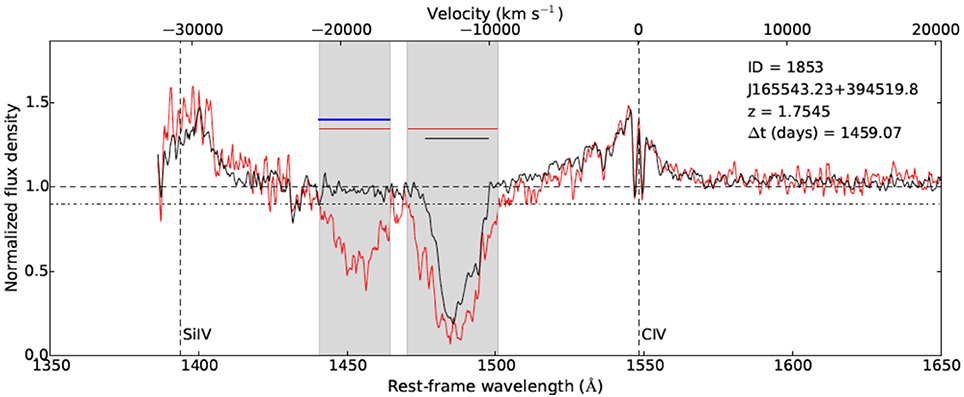
Figure 1. Overplot of a pair of SDSS-I/II (red) and BOSS (black) spectra showing a disappearing BAL trough and an additional non-disappearing BAL trough. We report the source ID in our catalog, the SDSS ID, the redshift, and the rest-frame time difference between the two spectra. Plots are limited to the wavelength window where C IV BAL disappearance can be observed. Horizontal axes: rest-frame wavelength (bottom) and velocity (top); vertical axis: normalized flux. Horizontal dashed line: normalized flux density = 1; dash-dot line: normalized flux density = 0.9. Vertical dashed lines: Si IV (1,394 Å) and C IV (1,549 Å) emission lines (rest-frame wavelengths). Red/black horizontal lines: BAL troughs in the SDSS-I/II/BOSS spectra; blue bars: SDSS-I/II BAL troughs that disappear in BOSS spectra. The regions corresponding to SDSS-I/II BAL troughs are shaded for better visualization.

For each source we perform a two-sample χ² test comparing the two sets of points corresponding to normalized flux density values in the SDSS-I/II and BOSS windows where we detect a disappearance (indicated by blue bars in Figure 1), and assume that a disappearance is reliable if the χ² test probability for the BAL variation to be not random is $P_{{\chi }^2}\le 10^{-4}$; this returns a sample of 67 sources with at least one C IV BAL trough that disappears in their spectra. Specifically, this sample includes three objects whose spectra show two C IV BALs that disappear, and two sources where the C IV disappearing BALs are three. This means that, in total, we detect 73 C IV disappearing BALs in the spectra of our sample of 67 sources. This means that in the BOSS spectra of the QSOs in our main sample we detect 1,801 (i.e., 1,874–73) C IV BAL troughs; specifically, if we consider the 67 sources for which we detect a disappearance, there are 40 of them whose BOSS spectra do not show any C IV BALs, and 27 of them where other C IV BAL troughs are still detected. As a consequence, the number of QSOs with C IV BAL troughs in their BOSS spectra is 1,279 (i.e., 1,319–40). We shall deal with the subsample of sources with additional non-disappearing BALs in section 3.3.

The average rest-frame time difference between two spectra where disappearance is observed is Δt is ≃1,123 days, corresponding to a timescale of ≈3.1 year. In Table 1 we gather together all the relevant numbers relative to our sources.

TABLE 1

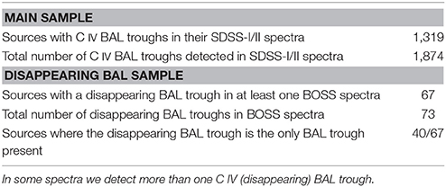
Table 1. Detailed information about our main sample of sources and the sample of C IV disappearing BAL troughs.

3.1. Lifetime Estimates

The fraction of disappearing BAL troughs is defined as the number of C IV BAL troughs that disappear in the BOSS spectra divided by the number of C IV BAL troughs detected in the SDSS-I/II spectra, i.e., $f_{\mathrm{\text{disapp}}}=73/1,874=3.9_{-0.5}^{+0.5}\%$. The fraction of QSOs with at least one disappearing BAL trough is defined as the number of QSOs where at least one disappearing C IV BAL trough is detected divided by the total number of QSOs where C IV BAL troughs are detected, i.e., f_QSO = 67/1,319 = ${5.1}_{-0.6}^{+0.7}\%$ (percentage errors are obtained following Gehrels, 1986, where approximated confidence limits are derived based on Poisson and binomial statistics). We can give an estimate of the average lifetime of a BAL trough along our line of sight as the maximum time difference between two epochs for each source divided by the fraction of BAL troughs disappearing over such time; we obtain ${\overline{t}}_{\mathrm{\text{trough}}}\approx \langle \Delta t_{\mathrm{\text{max}}}\rangle /f_{\mathrm{\text{disapp}}}=80_{-10}^{+10}$ year, the average value of the maximum time difference being 〈Δt_max 〉 ≈ 1,144 days.

Our estimate is roughly consistent with the orbital time (≈50 year; e.g., Filiz Ak et al., 2013, and references therein) of the accretion disk at distances where winds are thought to form, typically, i.e., ≈10⁻² pc; hence, disk rotation could possibly be the cause of BAL disappearance, and this may mean that BALs moving out of our line of sight will not be observable anymore, though they may still exist physically.

We know from the literature (e.g., Hall et al., 2002; Filiz Ak et al., 2012) that, if all the C IV BAL troughs in a spectrum disappear, there are generally no additional BALs left, meaning that the source is turned into a non-BAL QSO. In our sample there are 30 sources turning into non-BAL QSOs after their C IV BAL troughs disappear; the fraction of BAL QSOs changing into non-BAL QSOs is therefore f_transform = 30/1,319 = ${2.3}_{-0.4}^{+0.5}\%$. This allows us to estimate the lifetime of the BAL phase in a QSO, defined approximately as the aforementioned average of the maximum time difference between two epochs divided by the fraction of BAL QSOs that turn into non-BAL QSOs over that time span: ${\overline{t}}_{\mathrm{\text{BAL}}}\approx \langle \Delta t_{\mathrm{\text{max}}}\rangle /f_{\mathrm{\text{transform}}}\approx 136_{-24}^{+30}$ year. Again, we point out that our lifetime estimates are limited to what we see along our line of sight, but do not necessarily constrain the physical existence of a BAL, as it could simply move out of that direction. Also, we note that a BAL could emerge again in a region where a BAL previously disappeared, making the definition of BAL phase a tricky task.

Table 2 is a summary of the main numerical results of our analysis of C IV BAL trough disappearance.

TABLE 2

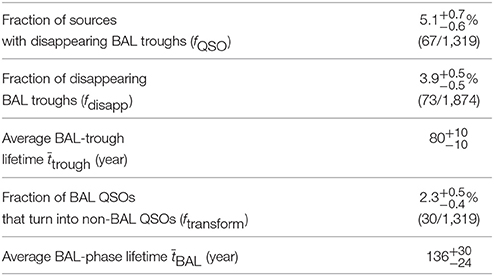
Table 2. Summary of our main numerical findings.

3.2. Velocity Distributions

BALs show some properties, in terms of their velocities, which can help characterize the BAL population. We compare the υ_max, υ_min, υ_c, and Δυ distributions for the disappearing BALs to the corresponding distributions for the whole main sample BALs and, on the basis of a Kolmogorov-Smirnov test comparing each pair (see Figure 2), we find that:

- the v_max distributions are not significantly different;

- the disappearing BALs generally have a high υ_min and central velocity;

- the disappearing BALs are generally narrow with respect to the whole sample of BALs.

FIGURE 2

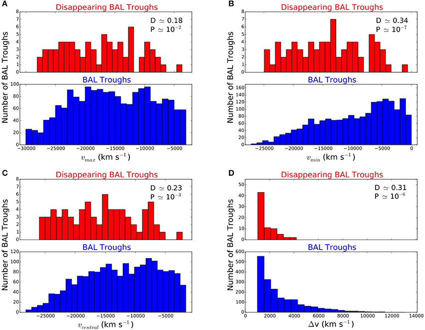
Figure 2. Maximum observed velocity υ_max (A), minimum observed velocity υ_min (B), central velocity υ_c (C), and BAL width Δυ (D) distributions for the sample of disappearing BAL troughs (upper red histogram in each panel) and for the main sample of BAL troughs (lower blue histogram in each panel). Results of the Kolmogorov-Smirnov test performed on each pair of cumulative distributions are reported in each panel: D is the maximum distance between the two cumulative distributions, and P is the probability to get a higher D value assuming that the two datasets are drawn from the same distribution function.

The distributions pairs show that disappearing BAL troughs are generally narrow and characterized by a higher outflow velocity than non-disappearing BALs. This last feature is confirmed by the analysis of the correlation in the variability of multiple BAL troughs in the same spectrum, discussed in next section. We used Kolmogorov-Smirnov test so that our findings can be easily compared to those by Filiz Ak et al. (2012), where part of our sample was analyzed; nevertheless, an Anderson-Darling test would probably be more suitable, as it is more sensitive on the distribution tails. We remind that this work is meant to be a preliminary version of a paper we are about to submit; more detailed results will be presented in the full paper. The results of our Kolmogorov-Smirnov tests are in agreement with the findings by Filiz Ak et al. (2012).

Figure 2 shows the various distribution pairs; in each panel we report the values of the two indicators obtained from the Kolmogorov-Smirnov test comparing each pair of cumulative distributions.

3.3. Correlation in BAL Variability

We already mentioned that sometimes there is more than one C IV BAL trough in a spectrum, and they do not necessarily disappear together. Additional non-disappearing BALs in spectra where we detect disappearing BALs can help us investigating the existence of a correlation in the variability of multiple BAL troughs in the spectra of a given source.

Our sample of 67 sources with disappearing BALs includes 27 objects for which we detect 28 additional non-disappearing BALs. Our investigation is limited to BAL troughs in SDSS-I/II spectra that correspond to BAL troughs in BOSS spectra; BALs turning into mini-BALs, or vice versa, are not taken into account. In all but one case, the disappearing BAL is the one with the higher central velocity. We compute the EW of these BALs from the same two spectra that allowed us to detect a disappearance, and compare them to the whole main sample of BALs, which is used as a reference population, as shown in Figure 3. We find that the main sample is characterized by symmetric variations in the EW, meaning they can get stronger as well as weaker, going from the less recent to the more recent epoch; conversely, $79_{-17}^{+21}\%$ (again, percentage errors are computed following Gehrels, 1986) of the additional non-disappearing BALs show a decreasing EW in the more recent spectrum, supporting the idea that some correlation between different BAL troughs in a spectrum exists. This seems to be a persistent phenomenon, concerning even BALs that are very distant from one another (central velocity offset up to ≈20,000 km s⁻¹).

FIGURE 3

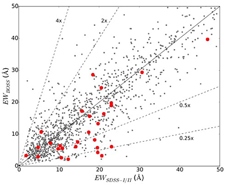
Figure 3. EWs at two different epochs for the sample of additional non-disappearing BALs in the spectra where disappearances are detected (large red dots). For each BAL trough, the two EWs are measured in the same epoch pair where disappearance is detected. Small gray dots in the background represent the EWs at two epochs (one from SDSS-I/II and one from BOSS) for all the sources in the main sample, measured from the most-recent SDSS-I/II epoch and the least-recent BOSS epoch for each source. The solid line indicates where the EWs of the two compared epochs are equal, while the dashed lines indicate where the EW of the BOSS epoch is four times, two times, half of, and a quarter of the EW in the SDSS-I/II epoch.

The explanation for such a correlation must be something global; the most accredited hypotheses attribute the observed correlation to variations in the density of the shielding gas, leading to changes in the ionizing flux reaching the absorbing gas and, hence, to variations in the ionization level of the absorbing gas. Nevertheless, recent works (e.g. Baskin et al., 2014) tend to favor models attributing the variations in the ionization level to the radiation pressure compression. However, it is likely that different causes contribute to the BAL variability phenomenon.

4. Future Perspectives

In the near future we would like to extend our analysis to lower ionization transitions, such as Si IV and Mg II, in order to investigate possible relations between the variability of troughs originating from different transitions; also, a parallel study of BAL emergence would be of interest in the framework of a thorough comprehension of the BAL phenomenon and their physics, structure, and evolution.

Author Contributions

All authors contributed to the design of the work, interpretation of data, drafting and revising of the work.

Funding

This paper is part of the “Quasars at all Cosmic Epochs” Research Topic and there are no publications fees for all participants to the conference. Publication fees were included in the conference fee and will be covered by the University of Padova.

Conflict of Interest Statement

The authors declare that the research was conducted in the absence of any commercial or financial relationships that could be construed as a potential conflict of interest.

Footnotes

1. ^The minus sign due to blueshift is not taken into account.

2. ^Throughout the present work we will refer to BAL QSOs and BAL troughs, and some clarification may be necessary: we define as BAL QSO each QSO whose spectrum exhibits at least one BAL trough, i.e., an absorption line having a width Δυ ≥ 2,000 km s⁻¹ and extending below 90% of the normalized continuum level. In some cases the BAL troughs detected in a spectrum are more than one. We remind the reader that the present work is focused on C IV BAL troughs.

References

Barlow, T. A. (1993). Time Variability of Broad Absorption-Line QSO's. Ph.D. Thesis, University of California.

Baskin, A., Laor, A., and Stern, J. (2014). Radiation pressure confinement - IV. Application to broad absorption line outflows. Mon. Not. Roy. Astron. Soc. 445, 3025–3038. doi: 10.1093/mnras/stu1732

CrossRef Full Text | Google Scholar

Capellupo, D. M., Hamann, F., Shields, J. C., Rodríguez Hidalgo, P., and Barlow, T. A. (2012). Variability in quasar broad absorption line outflows - II. Multi-epoch monitoring of Si IV and C IV broad absorption line variability. Mon. Not. Roy. Astron. Soc. 422, 3249–3267. doi: 10.1111/j.1365-2966.2012.20846.x

CrossRef Full Text | Google Scholar

Cardelli, J. A., Clayton, G. C., and Mathis, J. S. (1989). The relationship between infrared, optical, and ultraviolet extinction. Astrophys. J. 345, 245–256. doi: 10.1086/167900

CrossRef Full Text | Google Scholar

Dawson, K. S., Schlegel, D. J., Ahn, C. P., Anderson, S. F., Aubourg, É., Bailey, S., et al. (2013). The Baryon oscillation spectroscopic survey of SDSS-III. Astron. J. 145:10. doi: 10.1088/0004-6256/145/1/10

CrossRef Full Text | Google Scholar

Di Matteo, T., Springel, V., and Hernquist, L. (2005). Energy input from quasars regulates the growth and activity of black holes and their host galaxies. Nature 433, 604–607. doi: 10.1038/nature03335

PubMed Abstract | CrossRef Full Text | Google Scholar

Elvis, M. (2000). A structure for quasars. Astrophys. J. 545, 63–76. doi: 10.1086/317778

CrossRef Full Text | Google Scholar

Filiz Ak, N., Brandt, W. N., Hall, P. B., Schneider, D. P., Anderson, S. F., Gibson, R. R., et al. (2012). Broad absorption line disappearance on multi-year timescales in a large quasar sample. Astrophys. J. 757:114. doi: 10.1088/0004-637X/757/2/114

CrossRef Full Text | Google Scholar

Filiz Ak, N., Brandt, W. N., Hall, P. B., Schneider, D. P., Anderson, S. F., Hamann, F., et al. (2013). Broad absorption line variability on multi-year timescales in a large quasar sample. Astrophys. J. 777:168. doi: 10.1088/0004-637X/777/2/168

CrossRef Full Text | Google Scholar

Gehrels, N. (1986). Confidence limits for small numbers of events in astrophysical data. Astrophys. J. 303, 336–346. doi: 10.1086/164079

CrossRef Full Text | Google Scholar

Gibson, R. R., Brandt, W. N., Schneider, D. P., and Gallagher, S. C. (2008). Quasar broad absorption line variability on multiyear timescales. Astrophys. J. 675, 985–1001. doi: 10.1086/527462

CrossRef Full Text | Google Scholar

Gibson, R. R., Jiang, L., Brandt, W. N., Hall, P. B., Shen, Y., Wu, J., et al. (2009). A catalog of broad absorption line quasars in Sloan Digital Sky Survey data release 5. Astrophys. J. 692, 758–777. doi: 10.1088/0004-637X/692/1/758

CrossRef Full Text | Google Scholar

Green, P. J., Aldcroft, T. L., Mathur, S., Wilkes, B. J., and Elvis, M. (2001). A Chandra survey of broad absorption line quasars. Astrophys. J. 558, 109–118. doi: 10.1086/322311

CrossRef Full Text | Google Scholar

Grier, C. J., Brandt, W. N., Hall, P. B., Trump, J. R., Filiz Ak, N., Anderson, S. F., et al. (2016). C IV broad absorption line acceleration in Sloan Digital Sky Survey Quasars. Astrophys. J. 824:130. doi: 10.3847/0004-637X/824/2/130

CrossRef Full Text | Google Scholar

Grier, C. J., Hall, P. B., Brandt, W. N., Trump, J. R., Shen, Y., Vivek, M., et al. (2015). The Sloan Digital Sky Survey reverberation mapping project: rapid CIV broad absorption line variability. Astrophys. J. 806:111. doi: 10.1088/0004-637X/806/1/111

CrossRef Full Text | Google Scholar

Hall, P. B., Anderson, S. F., Strauss, M. A., York, D. G., Richards, G. T., Fan, X., et al. (2002). Unusual broad absorption line quasars from the Sloan Digital Sky Survey. Astrophys. J. Suppl. 141, 267–309. doi: 10.1086/340546

CrossRef Full Text | Google Scholar

Hewett, P. C., and Wild, V. (2010). Improved redshifts for SDSS quasar spectra. Mon. Not. Roy. Astron. Soc. 405, 2302–2316. doi: 10.1111/j.1365-2966.2010.16648.x

CrossRef Full Text | Google Scholar

Lundgren, B. F., Wilhite, B. C., Brunner, R. J., Hall, P. B., Schneider, D. P., York, D. G., et al. (2007). Broad absorption line variability in repeat quasar observations from the Sloan Digital Sky Survey. Astrophys. J. 656, 73–83. doi: 10.1086/510202

CrossRef Full Text | Google Scholar

Margala, D., Kirkby, D., Dawson, K., Bailey, S., Blanton, M., and Schneider, D. P. (2016). Improved spectrophotometric calibration of the SDSS-III BOSS Quasar sample. Astrophys. J. 831:157. doi: 10.3847/0004-637X/831/2/157

CrossRef Full Text | Google Scholar

Murray, N., Chiang, J., Grossman, S. A., and Voit, G. M. (1995). Accretion disk winds from active galactic nuclei. Astrophys. J. 451:498. doi: 10.1086/176238

CrossRef Full Text | Google Scholar

Pei, Y. C. (1992). Interstellar dust from the milky way to the magellanic clouds. Astrophys. J. 395, 130–139. doi: 10.1086/171637

CrossRef Full Text | Google Scholar

Peterson, B. M., Wanders, I., Bertram, R., Hunley, J. F., Pogge, R. W., and Wagner, R. M. (1998). Optical continuum and emission-line variability of Seyfert 1 galaxies. Astrophys. J. 501, 82–93. doi: 10.1086/305813

CrossRef Full Text | Google Scholar

Schlegel, D. J., Finkbeiner, D. P., and Davis, M. (1998). Maps of dust infrared emission for use in estimation of reddening and cosmic microwave background radiation foregrounds. Astrophys. J. 500, 525–553. doi: 10.1086/305772

CrossRef Full Text | Google Scholar

Sulentic, J. W., del Olmo, A., Marziani, P., Martínez-Carballo, M. A., D'Onofrio, M., Dultzin, D., et al. (2017). What does CIVλ1549 tell us about the physical driver of the eigenvector quasar sequence? Astron. Astrophys. 608:A122. doi: 10.1051/0004-6361/201630309

CrossRef Full Text | Google Scholar

Vanden Berk, D. E., Richards, G. T., Bauer, A., Strauss, M. A., Schneider, D. P., Heckman, T. M., et al. (2001). Composite quasar spectra from the Sloan Digital Sky Survey. Astron. J. 122, 549–564. doi: 10.1086/321167

CrossRef Full Text | Google Scholar

Weymann, R. J., Morris, S. L., Foltz, C. B., and Hewett, P. C. (1991). Comparisons of the emission-line and continuum properties of broad absorption line and normal quasi-stellar objects. Astrophys. J. 373, 23–53. doi: 10.1086/170020

CrossRef Full Text | Google Scholar

York, D. G., Adelman, J., Anderson, J. E. Jr., Anderson, S. F., Annis, J., Bahcall, N. A., et al. (2000). The Sloan Digital Sky Survey: technical summary. Astron. J. 120, 1579–1587. doi: 10.1086/301513

CrossRef Full Text | Google Scholar