A novel multiple objective optimization framework for constraining conductance-based neuron models by experimental data

Introduction

Conductance-based compartmental models are increasingly used in the simulation of neuronal circuits (Brette et al., 2007 ; Herz et al., 2006 ; Traub et al., 2005 ). The main challenge in constructing such models that capture the firing pattern of neurons is constraining the density of the various membrane ion channels that play a major role in determining these firing patterns (Bekkers 2000a ; Hille 2001 ). Presently, the lack of quantitative data implies that the density of a certain ion channel in a specific dendritic region is by and large a free parameter. Indeed, constraining these densities experimentally is not a trivial task to say the least. The development of molecular biology techniques (MacLean et al., 2003 ; Schulz et al., 2006 , 2007 ; Toledo-Rodriguez et al., 2004 ), in combination with dynamic-clamp (Prinz et al., 2004a ) recordings may eventually allow some of these parameters to be constrained experimentally. Yet to date, the dominant method is to record the in vitro experimental response of the cell to a set of simple current stimuli and then attempt to replicate the response in a detailed compartmental model of that cell (De Schutter and Bower, 1994 ; London and Hausser, 2005 ; Koch and Segev, 1998 ; Mainen et al., 1995 ; Rapp et al., 1996 ). Traditionally, by a process of educated guesswork and intuition, a set of values for the parameters describing the different ion channels that may exist in the neuron membrane is suggested and the model performance is compared to the actual experimental data. This process is repeated until a satisfactory match between the model and the experiment is attained.

As computers become more powerful and clusters of processors increasingly common, the computational resources available to a modeler steadily increase. Thus, the possibility of harnessing these resources to the task of constraining parameters of conductance-based compartmental models seems very lucrative. However, the crux of the matter is that now the evaluation of the quality of a simulation is left to an algorithm. The highly sophisticated comparison between a model performance and experimental trace(s) that the trained modeler performs by eye must be reduced to some formula. Previous studies have explored the feasibility of constraining detailed compartmental models using automated methods of various kinds (Achard and De Schutter, 2006 ; Keren et al., 2005 ; Vanier and Bower, 1999 ). These studies mostly focused on fitting parameters of a compartmental model to data generated by the very same model given a specific value for its parameters (but see (Shen et al., 1999 )). As the models that generated the target data contained no intrinsic variability, the comparison between simulation and target data was done on a direct trace to trace basis.

In experiments, however, when the exactly same stimulus is repeated several times, the voltage traces elicited differ among themselves to a significant degree (Mainen and Sejnowski, 1995 ; Nowak et al., 1997 ). Since the target data traces themselves are variable and selecting but one of the traces must to some extent be arbitrary, a direct trace to trace comparison between single traces might not serve as the best method of comparison between experiment and model. Indeed, this intrinsic variability (“noise”) may have an important functional role (Schneidman et al., 1998 ). Therefore, we propose extracting certain features of the voltage response to a stimulus (such as the number of spikes or first spike latency) along with their intrinsic variability rather than using the voltage trace itself directly. As demonstrated in the present study, these features can then be used as the basis of the comparison between model and experiment. Using a very different technique, yet in a similar spirit, (Prinz et al., 2003 ) segregated the behavior of a large set of models generated by laying out a grid in parameter space into four main categories of electrical activity as observed across many experiments in lobster stomatogastric neurons (see (Goldman et al., 2001 ; Prinz et al., 2004b ; Taylor et al., 2006 ).

We utilize an optimization method named multiple objective optimization (or MOO, Cohon, 1985 ; Hwang and Masud, 1979 ) that allows for several error functions corresponding to several features of the voltage response to be employed jointly and searches for the optimal trade-offs between them. Using this optimization technique, feature-based comparisons can be employed to arrive at a model that captures the mean of experimental responses in a fashion that accounts for their intrinsic variability. We exemplify the use of this technique by applying it to the concrete task of modeling the firing pattern of two electrical classes of inhibitory neocortical interneurons, the fast spiking and the accommodating, as recorded in vitro by (Markram et al., 2004 ). We demonstrate that this novel approach yields an excellent match between model and experiments and argue that the multiple, diverse models generated by this method for each neuron class (incorporating the inherent variability of neurons) could serve successfully as the building blocks for large networks simulations.

Materials and Methods

Every fitting attempt between model performance and experimental data consists of three basic elements: A target data set (and the stimuli that generated it), a model with its free parameters (and their range), and the search method. The result of the fitting procedure is a solution (or sometimes a set of solutions) of varying quality, as quantified by an error (or the distance) between model performance and the target experimental data.

Search Algorithm

Examples of search algorithms include, simulated annealing (Kirkpatrick et al., 1983 ), evolutionary strategies algorithms (Mitchell, 1998 ), conjugate-gradient (Press, 2002 ) and others. Cases of error functions comprise mean square error, trajectory density (LeMasson, 2001), spike train metrics (Victor and Purpura, 1996 ), and more (These two elements are by and large independent of one another i.e., almost any error function can be used by almost any search algorithm. Thus, we address the two issues separately).

In this study, we chose to use evolutionary algorithms. This class of algorithms was shown by Vanier and Bower (Vanier and Bower, 1999 ) to be an effective method for constraining conductance-based compartmental models. Our choice was motivated by the nature of these search algorithms that explore many solutions simultaneously and are naturally compatible with use on parallel computers. Briefly, an evolutionary algorithm is an iterative optimization algorithm that derives its inspiration from abstracted notions of fitness improvement through biological evolution. In each iteration (generation), the algorithm calculates the value of the target function (fitness) of numerous solutions (organisms). The set of all solutions (the population) is then considered. The best solutions are selected to pass over (breed) and be used in the next iteration. Solutions are not transferred intact from iteration to iteration but rather randomly changed (mutated) in various fashions. This process of evaluation, selection, and new solution generation is continued until a certain criterion for the quality of fitness between model performance and experimental results is fulfilled or the allotted iteration number has been reached. Among the many variants of such algorithms, we decided to use a custom made version of the elitist non-dominated sorting genetic algorithm (NSGA-II) (Deb et al., 2002 ) that we implemented in NEURON (Carnevale and Hines, 2005 ). We use real-value parameters. The mutation we used was a time diminishing non-uniform mutation (Michalewicz, 1992 ). Namely, the mutation changes the value of the current parameter by an amount within a range that diminishes with time (subject to parameter boundaries). The crossover scheme implemented is named simulated binary crossover (SBX) (Deb and Agarawal, 1995 ) and aims at replicating the effect of the standard crossover operation in a binary genetic algorithm. Thus, an offspring will have different parameter values taken from each of the two progenitors and some might be slightly modified. Lastly, we introduced a sharing function (Goldberg and Richarson, 1987 ) to encourage population diversity. This function degrades the fitness of each solution according to the number of solutions within a predefined distance. Thus, it improves the chances of a slightly less fit, yet distinct solution to survive and propagate. Our tests of different mutation and crossover operators show that these indeed affect the speed of progression toward good solutions but for most forms of operators the fitting eventually converged to similar degrees of success.

Error Functions

In this study, rather than suggesting a single optimal error function (which might not even be possible to define in the most general case), we adopt a strategy that allows several potentially conflicting error functions to be used jointly without being forced to assign a relative weight to each one. This method is entitled multiple objective optimization (Cohon, 1985 ; Deb, 2001 ; Hwang and Masud, 1979 ). It arose naturally in engineering where one would like to design, for instance, a steel beam that is both strong (one objective) and light (second objective). These two objectives potentially clash and are difficult to weigh a priori without knowing the precise trade-off.

In brief, an optimization problem is defined as a MOO problem (MOOP) if more than one error function is used and one considers them in parallel, not by simply summing them. The main difference between single objective optimization that has been previously used (Achard and De Schutter, 2006 ; Keren et al., 2005 ; Vanier and Bower, 1999 ) and the MOO is in the possible relations between two solutions. In a single objective problem, a solution can be either better or worse than another, depending on whether its error value is lower or higher. This is not the case in multiple objective problems. The relation of better or worse is replaced by that of domination. One solution dominates another if it does better than the other solution in at least one objective and not worse than the other solution in all other objectives. If there are M objective functions fj(x), j…M, then a solution x¹ is said to dominate a solution x² if both the following conditions hold,

Thus, one solution can dominate a second one, the second can dominate the first, or neither dominates each other. Solutions are found to not dominate each other when each is better than the other in one of the objectives but not in all of them. In other words, solutions do not dominate each other if they represent different trade-offs between the objectives. Indeed, the goal of a MOOP is to uncover the optimal trade-offs between the different objectives (termed the pareto front, derived from pars meaning equal in Latin) see Figure 4 .

Feature-based Error Functions

The multiple objectives we used are features of the spiking response such as spike height, spike rate, etc. (see below). The error functions we employ can, therefore, be termed feature-based error functions. The error value is calculated as follows: for a given stimulus (e.g., depolarizing current step) the value of each feature is extracted for all experimental repetitions of that stimulus. The mean and standard deviation (SD) of the feature values is then computed. Given the model response to that same stimulus, the value of the feature is extracted from the model as in the experimental trace. Then the difference between the mean value of the experimental responses and that of the model response is measured in units of the experimental standard deviation. This is used as the error value for this feature. For instance, if the feature considered is the number of action potentials (APs) and the experimental responses to the stimulus elicited on average seven APs with a standard deviation of 1, then a model with eight APs would have an error of 1. Similarly, if the feature considered is the mean spike width which is experimentally, on average across repetitions, 1 ms with SD of 0.2 ms, and the mean spike width in the model is 1.4 ms, then the error in this case is 2. An error of 0 in all features would mean a full match between model performance and average experimental behavior.

The error functions we chose for the present study consist of six features extracted from the response of cortical interneurons to suprathreshold depolarizing step currents: (1) spike rate; (2) an accommodation index; (3) latency to first spike; (4) average AP overshoot; (5) average depth of after hyperpolarization (AHP); (6) average AP width (Figure 2 ).

Spike rate is calculated by dividing the number of spikes in the trace by the duration of the step current (2 seconds). The accommodation index is defined by the average of the difference in length of two consecutive inter-spike intervals (ISIs) normalized by the summed duration of these two ISIs. It is along the lines of previously developed measures of accommodation. Specifically, the local variance introduced by (Shinomoto et al., 2003 ). The equation for the accommodation index is as follows;

Where N is the number of APs and k determines the number of ISIs that will be disregarded in order not to take into account possible transient behavior as observed in (Markram et al., 2004 ). The value of k was either four ISIs or one-fifth of the total number of ISIs, whichever was the smaller of the two. Latency to first spike is the time between stimulus onset and the beginning of the first spike (defined as the maximum of the second derivative of voltage). Average AP overshoot is calculated by averaging the absolute peak voltage values of all APs. Average AHP depth is obtained by the mean of the minimum of the voltage trough between two consecutive APs. Average AP width is calculated by averaging the width of every AP at the midpoint between its onset and its peak. A schematic portrayal of the extraction of these features is shown in Figure 2 .

For each of the two neuron classes modeled, we injected three levels of depolarizing current as in the experiments. For a given stimulus strength, the error between model and experiments was calculated for each feature. The final error value for each feature was the average of the errors calculated over the three levels of current pulses.

Cell Model

Simulations were performed using NEURON 5.9 (http://www.neuron.yale.edu ; Carnevale and Hines, 2005 ). The cell used as the basis for the model was a reconstructed nest basket cell interneuron (Figure 1 C). The model was composed of 301 compartments. Voltage-dependent ion channels were inserted only at the model soma; for simplicity dendrites and axon were considered to be passive. Dynamics of the ion channels were taken from the experimental literature (see below). When possible they were obtained from studies performed on cortical neurons. Ion channels were kept in their original mathematical description. The value for the maximal conductance of each ion channel type was left as a free parameter to be fitted by the MOO algorithm. The 10 ion channels that were used are listed below along with the bounds of the maximal conductance. The lower bound was always zero. The upper bound (UB) was selected based on estimates on reasonable physiological bounds and later verified by checking that the acceptable solutions of the fitting are not affected by increasing the UB value. Unless otherwise noted, UB was 1000 mS/cm².

The following ion channels were used: persistent sodium channel, Na_p (Magistretti and Alonso, 1999 ); UB = 100 mS/cm². All upper bounds following will be in the same units. Fast inactivating sodium channel, Na_t (Hamill et al., 1991 ); Fast-inactivating potassium channel, K_fast (Korngreen and Sakmann, 2000 ); Slow inactivating potassium channel, K_slow, (Korngreen and Sakmann, 2000 ); A-type potassium channel I_A (Bekkers, 2000b ); Fast non-inactivating Kv 3.1 potassium channel, Kv3.1 (Rudy and McBain, 2001 ); M-type potassium channel I_m (Bibbig et al., 2001 ); UB 100. High-voltage-activated calcium channel, Ca (Reuveni et al., 1993 ); UB 100. Calcium dependent small-conductance potassium channel, SK (Kohler et al., 1996 ); UB 100. Hyperploarization-activated cation current I_h (Kole et al., 2006 ); UB 100.

We found that the range of the window current of the transient sodium channel was too hyperpolarized for fitting the AP features. Consequently, the voltage-dependence of this channel was shifted by 10 mV in the depolarized direction. For the same reason, the voltage-dependence of the K_slow channels was shifted by 20 mV in the depolarized direction.

The MOO algorithm was run on parallel computers, either on a cluster consisting of 28 Sun x4100, dual AMD 64 bit Opteron 280 dual core (total of 112 processors), running Linux 2.6, or on a Bluegene/L supercomputer (Adiga et al., 2002 ). Average run time of a single fitting job on the cluster was less than 1 day. Runtime on 256 processors of the Bluegene/L was roughly equivalent to that of the cluster. Nearly linear speedup was achieved for 512 processors by allowing multiple processors to simulate the different step currents of the same organism.

Convergence of Fitting Algorithm

The parameter set of the fitting consisted of 12 parameters; the maximal conductance of the 10 ion channels mentioned above and the leak conductance in both the soma and the dendrites. Each run consisted of 300 organisms (300 sets of parameter values evaluated at each iteration). The design of the genetic algorithm causes the best fit for each objective to survive from generation to generation (see above). This ensures that the fit at each succeeding generation is no worse than that in the previous one. Our stop criterion for fitting was the number of iterations which is always 1000 in this study. We found that in our case, different choices in the same range of values (e.g., 1200 iterations and 350 organisms) did not lead to different results. Even significant changes in these values (2000, 4000, 8000 iterations) do not lead to qualitatively different outcomes. For each electrical class, the fitting was repeated several times using different random seeds. Different seeds result in different initial conditions and dissimilar choices in the stochastic search of the algorithm. The end results of runs with different seeds did not produce qualitatively dissimilar results.

Experimental Data

The firing response of two classes of inteneurons, fast spiking and accommodating were taken from in vitro recordings of the rat somatosensory cortex. The experimental procedures were published in (Markram et al., 2004 ). Two cells, one fast spiking and the other accommodating, were selected from our large experimental database. For each cell, we selected 15 voltage traces (each 3 seconds long); five repetitions for each of three levels of depolarizing step currents (150, 225, and 300 pA). For each stimulus strength, the mean and SD for each of the six features (see above) was calculated; a summary is provided in Tables 1 2 3 .

TABLE 1

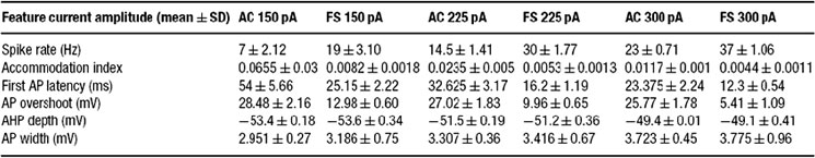
Table 1. Feature-based error targets for accommodating (AC) and fast spiking (FS) cortical intemeurons.

TABLE 2

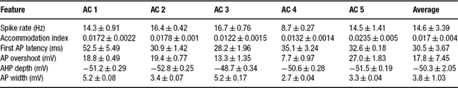
Table 2. Feature statistics for five accommodating interneurons (current input, 225 pA).

TABLE 3

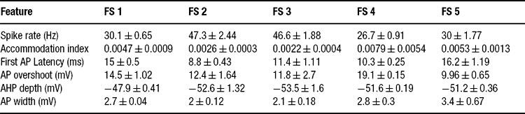
Table 3. Feature statistics for five fast spiking interneurons (current input, 225 pA).

Results

Figure 1 depicts the exemplars of the two classes that were the targets of the fitting. In order to demonstrate the intrinsic variability that these neurons exhibit for a repeated (frozen) input, two repetitions of the same 2 second long, 150 pA depolarizing current are displayed for each class. Note the difference in the two traces within class, albeit the fact that the exactly same stimulus was given in the two cases. Our fitting method, therefore, aims at capturing the main features of these responses rather than targeting a specific trace (see Methods).

FIGURE 1

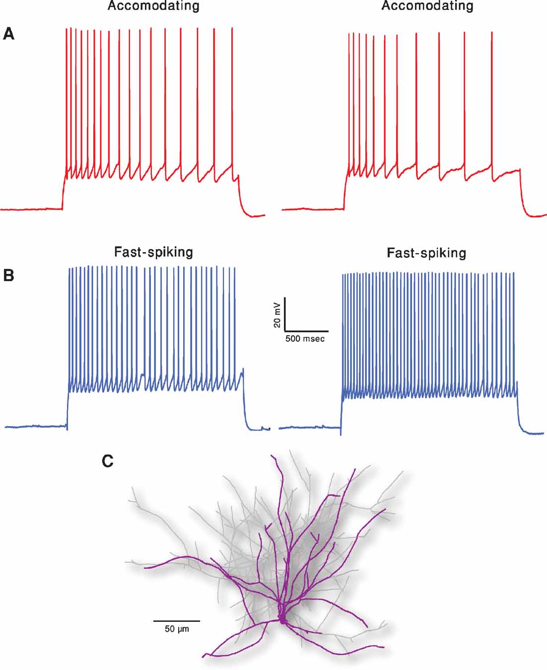
Figure 1. Two classes of firing patters in cortical interneurons. (A) Accommodating interneuron (red traces). Two experimental responses of the same cell to a 2 seconds long, 150 pA depolarizing current. Time elapsed between the two responses is 10 seconds. (B) Fast spiking interneuron (blue traces). Same current input as in A. Membrane potential of all cells was shifted to –70 mV prior to the current step injections. Note that these two exemplars of the electrical classes are clearly distinct and that, for a given cell, there is a considerable variability between traces although the current input remains exactly the same (e.g., number of spikes and spike timing). (C) Reconstructed nest basket cell interneuron used for simulations. Dendrites are marked in purple and axon in light gray.

The six different features chosen in the present study to characterize the firing patterns are depicted in Figure 2 . Their corresponding experimental target values (mean ± SD) for the two classes is summarized in Table 1 . As can be seen in this table, the values of some of these features are clearly distinct between the two classes, supporting the possibility that the fitting procedure will give rise to two different models (with different sets of maximal conductances for the different ion channels current chosen, see Methods) for these two different classes.

FIGURE 2

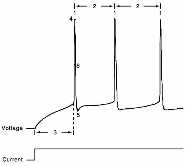
Figure 2. Feature extraction. Voltage response (top) to a step depolarizing current (bottom) of the first 200 ms following stimulus onset of the trace displayed in Figure 1 A. Extraction of the six features is schematically portrayed. 1, spike rate; 2, accommodation index (Equation 3); 3, latency to first spike; 4, AP overshoot; 5, After hyperpolarization depth; 6, AP width. For values of the different features in the case of the two electrical classes depicted in Figure 1 , see Table 1 .

Table 2 shows the mean and variability of the features for the neuron selected as the exemplar of the accommodating class (AC 5) alongside four other neurons of the same class. Also given for each feature are the class statistics obtained by taking the mean of each of the five neurons as a single sample. As can be seen, the exemplar represents the class rather faithfully, with somewhat more pronounced accommodation.

All that the algorithm requires are the target statistics–the mean and SD of the different features. Thus, one can create a model based on the statistics of each individual cell separately, or fit directly the general class statistics. We find that the algorithm managed to fit all of the single neuron statistics presented here as well as the class statistics. Table 3 shows the equivalent of Table 2 for the fast spiking class. As can be seen, the spike rate feature is quite variable in this class.

In Figure 3 , the results of our fitting procedure are demonstrated for the exemplars of the two electrical classes (AC 5, FS 5). In Figure 3 A, we plot the progression of error values with generation for the accommodating behavior. The error (y-axis) is composed of the sum of errors for six features and is thus six-dimensional. In order to simplify the graph, the error values for the six features are weighted equally and summed to yield a single error value. In this graph, the error value of the organism with the minimal error of the total of the 300 evaluated in each generation is plotted. Three repetitions of the fitting with different random seeds are shown. In the three cases, the final iterations all converge to a similar error value ranging between 5 and 7 (red error at right). This means that, on average, every evaluated feature of the best model fell within one SD of the experimental traces.

FIGURE 3

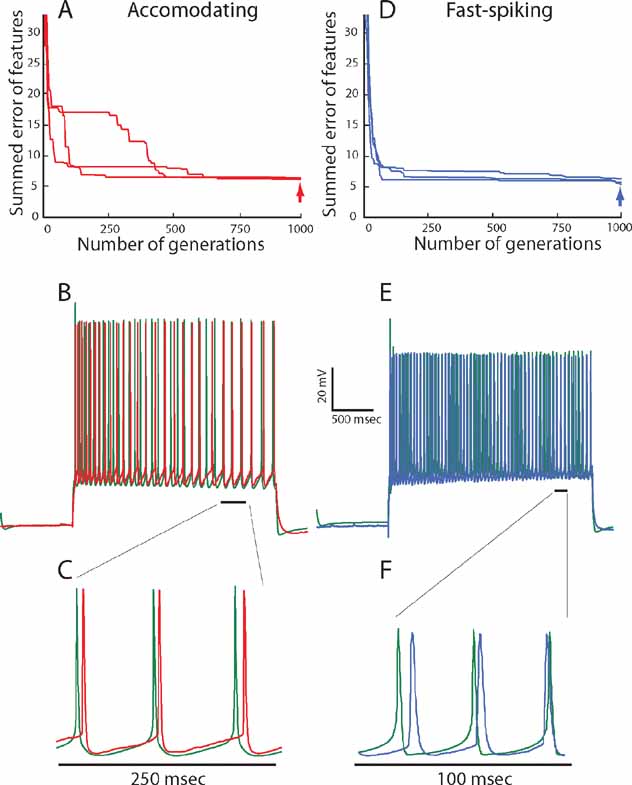
Figure 3. Fitting of model to experimental traces using multi-objective optimization procedure. (A) Convergence of summed errors for the accommodating behavior with generation. Errors for the six objectives (in SD units) are weighted equally and summed to a single error value. In each generation, 300 sets of parameter values (values for maximal ion conductance) are evaluated simultaneously. The error value for the set of parameters that yield the minimal error is plotted. The three lines show the same fitting procedure repeated using different random initial conditions. (B) Comparison between one of the experimental responses (red) of the accommodating neuron shown in Figure1 A, to a 225 pA, 2 seconds depolarizing current pulse and the model response (green trace) to the same input, using the best set of ion channel conductances obtained at the 1000th generation (point denoted by red arrow in A). The values of the channel conductances (in mS/cm²) obtained in this fit are: Na_t = 359; Na_p = 0.00033; K_fast = 423; K_slow = 242; I_A = 99; Kv3.1 = 218; Ca = 0.00667; SK = 32.8; I_h = 10; I_m = 0; Leak_soma = 0.00737; Leak_dendrite = 0.001. (C) Zoom into the region marked by a black line in B. (D) Convergence of summed errors for the fast-spiking behavior for the six objectives with generation as in A. (E) Comparison between one of the experimental responses (blue) of the fast-spiking neuron shown in Figure 1 B, to a 225 pA, 2 seconds depolarizing current pulse and the model response (green trace) to the same input, using the best set of ion channel conductances obtained at the 1000th generation (point denoted by blue arrow in D). The values of the channel conductances (in mS/cm²) for this fit are: Na_t = 172; Na_p = 0.1; K_fast = 0.5; K_slow = 199; I_A = 51; Kv 3.1 = 89; Ca = 0.00153; SK = 97; I_h = 4; I_m = 64; Leak_soma = 0.06; Leak_dendrite = 0.00163. (F) Zoom in to the region marked by a black line in E.

Figure 3 B shows a response of the model that had the lowest error value at the last iteration to a 225 pA, 2 ms long depolarizing current pulse to allow a visual impression of the fit (experimental response in red and model in green). As can be seen, though the model was never directly fit to the raw voltage traces, the resulting voltage trace closely resembles the experimental one. Indeed, zooming in into these traces (Figure 3 C) shows that the general shape of the AP (its height, width, AHP depth) looks very similar when comparing model and experiments. The same close fit between model and experiments is also obtained for the other class–the fast spiking interneuron (Figures 3 D-F).

Regarding the quality of fit, one may see that the algorithm manages to find a good, but not perfect match to both target interneuron electrical behaviors. As stated previously, when one wishes to fit experimental data with a limited set of channels, not finding a perfect fit is hardly surprising. This could be due to inaccuracies in the experimentally derived dynamics of the channels or due to the fact that the real cell might contain on the order of tens of channels inhomogenously distributed across the surface of the dendrite and the model contains only 10 channels distributed over the soma and a passive leak current in the dendrite and axon. It is also important to note that there are a few significant deviations between the model derived from the feature-based error and the experimental traces. This is most marked in the height of the first spike (see for instance Figures 3 B and 3 E). This could have been addressed by modifying the details of the experimentally found Na_t channel dynamics but we chose not to do so.

Using MOO, we are interested in exploring the best possible trade-offs between objectives as found at the end of the fitting procedure. In order to visualize this, the value of the error of each of the M different objectives should be plotted against the error in the other objectives. In Figure 4 , we project this M-dimensional error space into a two-dimensional space, choosing two examples (Figures 4 A and 4 B) out of the total of M choose 2 possible examples. Three hundred organisms (parameter sets) of the fitting of the accommodating behavior at the final iteration (number 1000) are shown. The line connecting the error values of the solutions that do not dominate each other (and thus represent the best tradeoffs) is the pareto front (black dashed line). The line is obtained by finding the solutions that do not dominate each other (for definition, see Methods) and connecting them by a line (in two-dimensional space or the equivalent manifold in higher dimensional space).

The goal of the fitting procedure was to minimize each of the error values. Though the full error and hence also the pareto front reside in six-dimensional case, in order to visualize the pareto front, let us consider the full error to consist of solely the two-dimensional projection under consideration. Under that assumption, in the two-dimensional plot, the best result would be to have points whose value is as close to zero in both the x and y dimensions. If a value of zero cannot be simultaneously reached in both dimensions, then the exact nature of the trade-offs between the two plotted error functions, i.e., the shape of the pareto front, becomes of interest. While the shape of the front can be quite arbitrary, it is useful to consider two different boundary cases in two dimensions. One is the case in which there is no effective trade-off between the two objectives (accommodation index vs. AP overshot, Figure 4 A). In this case, in the left part of Figure 4 A, the pareto front is almost parallel to the y-axis. Thus, for the lowest value of the error in the AP overshoot (the x-axis) there is a range of both high and low error values for the accommodation index (y-axis). Naturally, the desired value would be that with the lowest error in the y-axis. The same holds mutatis mutandis when one considers the x-axis, as the pareto front in its lower part is parallel to the x-axis. Hence, the best solution is clearly that in the lower left corner (black arrow). Note that as a minimum in both error values can be achieved simultaneously there is no effective trade-off between the two objectives. In this case, the lower left point in the pareto front would also be the optimal solution for weighted sums of the two objectives also when the weighting of the two errors is not identical.

FIGURE 4

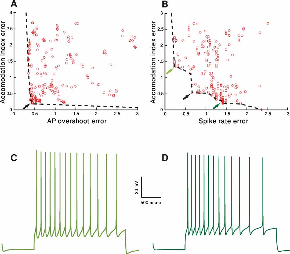
Figure 4. Objective tradeoffs–the pareto fronts. A-D. Fitting of the accommodating neuron displayed in Figure 1 A. In both A and B, for each of the 300 parameter sets in the 1000th generation, the final error values (in SD units) of two (out of the total of six) objectives (features) are plotted against each other. Each circle represents the error resulted from a specific parameter set. The set of error values that provided the best trade-offs between the two objectives are connected with a black dashed line (the pareto front, see Methods). Black arrows represent the errors corresponding to the solution depicted in Figures 3 B, 3 C. (A) AP overshoot versus accommodation index. (B) Accommodation index vs. spike rate. (C) Model response to 150 pA, 2 seconds depolarization using the error values marked in B by the light green arrow at top left. The values for the channel conductances (in mS/cm²) in this case are: Na_t = 305; Na_p = 0.00565; K_fast = 38; K_slow = 277; I_A = 19; Kv3.1 = 6; Ca = 0.00477; SK = 49; I_h = 2; I_m = 0; Leak_soma = 0.0044; Leak_dendrite = 0.001. (D) Model response to 150 pA, 2 seconds depolarization, using the error values marked in B by the dark green arrow at bottom right. The values of the channel conductances (in mS/cm²) in this case are: Na_t = 389; Na_p = 0; K_fast = 29; K_slow = 175; I_A = 122; Kv3.1 = 42; Ca = 0.00606; SK = 41; I_h = 9; I_m = 0; Leak_soma = 0.0034; Leak_dendrite = 0.001.

In contrast, the pareto front in Figure 4 B (accommodation index vs. spike rate) is not parallel to the axes. Thus, some of the points along its perimeter will have lower values of one feature but higher values of the other one (e.g., the points marked by the three arrows). As the minimal value of one feature can be achieved only by accepting a value of the other objective higher than its minimum value, some trade-off exists between these two features. Therefore, different decisions on the relative importance of the two features will result in different points on the pareto front considered as the most desired model. Accordingly, if one wishes to sum the two errors and sort the solutions on the pareto front by the value of this sum, different weighings of the two objectives will result in different models considered as the minimum of the sum. The black arrow in Figure 4 B marks the point considered to be the minimum by an equal weighting. Alternatively, putting more emphasis on the error in spike rate (x-axis) would select a point such as that marked by the light green arrow (top-left). Conversely, weighing the error in accommodation (y-axis) more heavily will favor a point such as that marked by a dark green arrow (bottom-right).

Figures 4 C and 4 D serves to demonstrate the effect of selecting different preferences regarding the two features. Figure 4 C shows the response of the model that corresponds to the error values marked by a light green arrow in Figure 4 B (upper-left) and Figure 4 D shows the model response corresponding to the error marked by the dark green arrow (lower-right), both to a 150 pA, 2 seconds depolarizing step current. As can be seen, spike accommodation of the light green model trace (Figure 4 C) is less pronounced than that of the dark green model trace (Figure 4 D). This is the reflection of the fact that the error value for accommodation of the dark green model is smaller than that of the light green model. On the other hand, in the light green model, more weight was given to the spike rate feature. Indeed, the light green trace has 14 APs (exactly corresponding to the experimental mean rate of seven spikes per second) while the dark green has only 13 APs. Note that similar variability as depicted in these two model-generated green traces may be found in the experimental traces for the same cell and same depolarizing step. The light green model trace is more reminiscent of the first experimental trace of the accommodating cell (Figure 1 A upper-left) whereas the dark green trace is more similar to the second (Figure 1 A upper-right).

Figure 5 portrays the spread of model parameter values at the end of the fitting for both electrical classes (red–accommodating; blue–fast-spiking). Each of the 300 parameter sets (each set composed of 12 parameters–the maximal conductance of the different ion channels) at the final iteration of a fitting that passes a quality criterion is represented as a circle. The criterion in this case was an error of less than 2 SD in each feature. The circle is plotted at a point corresponding to the value of the selected channel conductance normalized by the range allowed for that conductance (see Methods). Since there are 12 parameters, it is difficult to visualize their location in the full 12-dimensional space. Thus, for illustration, we project the parameter values of all models onto a three-dimensional subspace (Figures 5 A and 5 B) and to one-dimensional space for each of the 12 parameters (Figure 5 C). Note that many solutions overlap. Hence, the number of circles (for each class of firing types) might seem to be smaller than 300. In Figure 5 D, a subset of only seven solutions depicted in Figure5 C is displayed with different colored lines connecting the parameters values of each acceptable solution.

FIGURE 5

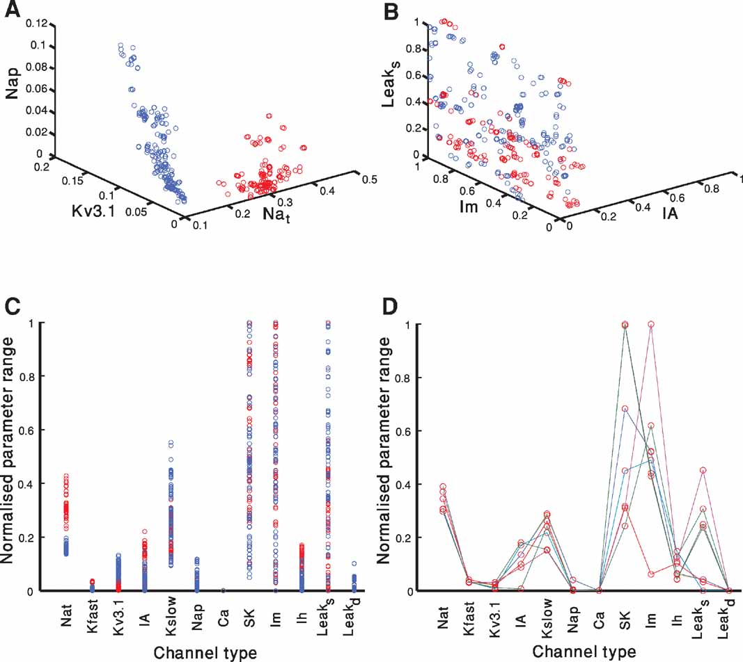
Figure 5. Parameter values of acceptable solutions. A-B. Each of the 300 parameter sets at the final iteration of a fitting attempt that has an error of less than 2 SD in each objective is represented as a circle. The circle is plotted at the point corresponding to the normalized value of the selected channel conductance. Red circles represent models of the accommodating neuron and blue represent models of the fast-spiking neuron. Plotted are the results of two out of the three repetitions of the fitting attempt shown in Figure 3 . (A) The channels selected were: Na_t, Na_p , Kv3.1. (B) The channels selected were: Leak_soma, I_m, I_A. (C) As in A and B, but here each of the parameter set for each of the 300 acceptable solution at the 1000th generation is depicted as a circle on a single dimensional plot. The circle is plotted at the point corresponding to the normalized value of the channel conductance. Note that even when projected onto a single dimension the two electrical behaviors occupy separate regions for some of the channels. (D) A subset of seven of the parameter sets of the accommodating behavior displayed in red in B is depicted. Lines connect each set of parameters that correspond to an acceptable solution. Thus, each individual line represents the full parameter set of a single model.

A few observations can be made considering Figures 5 A-C. First, there are many combinations of parameters that give rise to acceptable solutions (i.e. non-uniqueness, see (Golowasch et al., 2002 ; Keren et al., 2005 ; Prinz et al., 2003 ) and see below). Second, confinement of the parameters for the two different modeled classes (red vs. blue) to segregated regions of the parameter space can be seen both in the three-dimensional space (Figure 5 A) and even in some of the single dimensional projections (for instance Na_t in Figure 5 C). While for other subspaces, both in three dimensions (Figure 5 B) and single dimensions (for instance I_m in Figure 5 C), the regions corresponding to the electrical classes are more intermixed. Third, for some channel types, successful solutions appear all across the parameter range (e.g., SK or I_m) whereas for other channel types (e.g., I_h or K_fast) successful solutions appear to be restricted to a limited range of parameter values.

Figure 6 portrays the experimental (red) versus model (green) variability. The source of the variability of the in vitro neurons is most likely due to the stochastic nature of the ion channels (Mainen and Sejnowski, 1995 ; Schneidman et al., 1998 ). In contrast, the in silico neurons are deterministic and have no internal variability. Yet, if one considers the full group of models generated to fit one cell, differences in the channel conductances may bring about similar variability. Thus, even though the sources of the variability are disparate, the range of models may be able to capture the experimental variability. As the number of repetitions performed experimentally was low, we normalize the values of the different repetitions of each cell to the mean and SD of that cell and pool all five cells together. As can be seen in Figure 6 , the models (green circles) manage to capture nearly the entire range of experimental variability (red circles) with minimal bias.

FIGURE 6

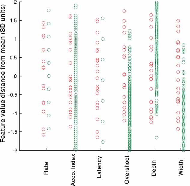
Figure 6. Experimental versus model variability–accommodating neurons. For each of the five cells shown in Table 2 , the values of each feature for the 225 pA step current is extracted for all repetitions. The mean of the feature value for each cell is subtracted and the result divided by the SD to arrive at the normalized distance from mean. All repetitions of all five accommodating cells have been pooled together and are displayed for each feature separately (red circles). The same process is repeated for the single repetition available for each of the 300 parameter sets that passed the 2 SD criterion (green circles) at the end of the fitting process of the accommodating exemplar (AC 5 Table 2 ).

Discussion

In this study, we have proposed a novel framework for constraining conductance-based compartmental models. Its central notion is that rather than trying to reduce the complex task of automated comparison between experimental firing patters of neurons and simulation results to a single distance parameter, one should adopt a multiple objective approach. Such an approach enables one to employ jointly more than a single error function, each comparing a different aspect (or feature) of the experimental and model data sets. Different features of the response (e.g., spike rate, spike height, spike timing, etc.) could be chosen according to the aim of the specific modeling effort. The mean and SD of each feature is then extracted from the noisy experimental results, allowing one to assess the quality of the match between model and experiment in meaningful units of the experimental SD. This framework generates a group of acceptable models that collectively represent both the mean and the variance of the experimental dataset. Whereas each individual model is still deterministic and will represent only a single instance of the experimental response, as a group the models capture the variability found experimentally.

Single Versus Multiple Objective Optimization

In order to assess the quality of the match between two voltage traces (e.g., experimental vs. simulated) that exhibit spiking behavior, different distance functions have been considered (Keren et al., 2005 ; Victor and Purpura, 1996 ). These studies seek for a single error function to describe the quality of the match between the two traces. However, given the complicated nature of this comparison, one distance function might not suffice. For instance, while the trajectory-density error function accounts for the form of the voltage trace it excludes the time parameter (LeMasson and Maex, 2001 ). Yet, one would also like to capture aspects of timing such as the first spike latency or the degree of accommodation. In order to accomplish this, an additional error function must be introduced. One may still sum these different error functions to obtain a single value (Keren et al., 2005 ); however, this potentially makes it difficult to have the different error functions contribute equally to the sum, as there is no guarantee that the error values are in the same range or magnitude. Hence, they would require being normalized one against the other. The problem is even more acute if one wishes to fit multiple stimuli with multiple error functions.

Even if the above-mentioned normalization can be accomplished, the relative contribution of each of the error functions to the final error value must be assigned when they are summed. Yet, it seems very difficult to assign a specific value to the relative importance of two different stimuli, for instance, a depolarizing ramp and depolarizing step current. How would one decide which of them should contribute more to the overall error? Lastly, one must also account for the fact that different models are used for different purposes, placing emphasis on diverse aspects of the model. For instance, in some cases it might be particularly important to match the first spike latency as accurately as possible (e.g., in models of the early visual system) while in other cases one might assign more importance to the overall spike rate. Using MOO, the error values of different error functions need not be summed and the problem of error summation is never encountered.

Feature-based Error Functions

We opted for feature-based error functions for suprathreshold depolarizing current steps for three main reasons. (i) Their ability to take into account the experimental intrinsic variability; (ii) the clear demarcation of the electrical classes that they provide (Table 1 ); and (iii) the ease of interpreting the final fitting results (i.e., the errors measured in SD that have a direct experimental meaning). Of course, using MOO one can employ any combination of direct comparison (e.g., mean square error) and feature-based error functions without being concerned by the fact that they return very different error values.

While MOO provides clear advantages over single objective optimization, the choice of the appropriate error functions must still be guided by the specific modeling effort. Different stimuli will be well addressed by different error functions. For instance, though mean square error is well known to be a poor option for depolarizing step currents that cause the model to spike (LeMasson and Maex, 2001 ), it is a reasonable measure when the stimulus is a hyperpolarizing current.

The main disadvantage of direct comparison (as opposed to feature-based errors) is the difficulty to incorporate the intrinsic variability of the experimental responses. Calculating the mean of the raw voltage responses will result in an unreasonable trace and any selection of a single trace must be to some degree arbitrary. A second disadvantage is the fact that direct comparison assigns an equal weight to every voltage point which might lead to unequal weighting of different features. For instance, the peak of a spike will be represented by very few voltage points (as it is brief in time) while the AHP will include many more points. Thus, a point-by-point comparison will allot more weight to a discrepancy in the AHP depth than in the AP height. A final disadvantage is that the error value returned by a direct comparison is an arbitrary number that is difficult to interpret. This makes judging the final quality of a model a complicated matter.

Interpreting the End Result of a Multi-objective Fitting Procedure

At the end of a MOO fitting procedure, one is presented with a set of solutions. For each of the solutions, the value of the different parameters (in our case the maximal conductance of the channel types) and the error values for all features are provided. After a threshold for the acceptance of solution is selected (e.g., an error of two SDs or less) one remains with a set of points, in parameter and error space, deemed successful that must be interpreted.

The location of successful solutions in error space can be used to plot the pareto fronts that in turn map which objectives are in conflict with one another. This allows one to pinpoint where the model is still lacking (or which combination of objectives yet presents a more significant challenge for the model). The nature of the conflicting objectives might also suggest what could be modified in the model to overcome this conflict. For instance, if the value of the AHP is in conflict with the number of spikes, perhaps one type of potassium channel is determining both features, and thus another type of potassium channel may be added to allow minimization of the error in the two objectives simultaneously. Note that this type of information is completely lost if one uses single-objective optimization. Furthermore, knowing which objectives are in conflict with one another is particularly important if one wishes to collapse two objectives into one by summing their corresponding error values. As noted in Figure 4 above, if objectives are not conflicting, then their exact relative weighting will not drastically affect the point considered as a minimum of their sum. However if they are conflicting an algorithm that tries to minimize their sum will be driven toward different minima according to the weighting of the objectives.

One may employ the spread of satisfactory models in parameter space to probe the dynamics underlying the models of a given electrical class. Yet, the functional interpretation of the spread of maximal conductance of channels for all acceptable solutions across their allowed range is not trivial (Figure 5 ) (Prinz et al., 2003 ; Taylor et al., 2006 ). One basic intuition is that if the value of a parameter is restricted to a small range then the channel it represents must be critical for the model behavior. Conversely, if a parameter is spread all across the parameter range, i.e., acceptable solutions can be achieved with any value of this parameter, the relevant channel contributes little to the model dynamics. Care should be taken when following this intuition since the interactions between the different parameters must be taken into account. For instance, if the model behavior critically depends on a sum of two parameters rather than their individual values (e.g., Na + K conductances) then the sum could be achieved by many combinations. Thus, while each of these channels is critical, the range of their values across successful solutions might be quite wide. Similar considerations hold for different types of correlations between the variables.

With the caveat mentioned above, it is still tempting to assume that those parameters that have different segregated values in parameter space are those that are responsible for the difference in the dynamics of the two classes (accommodating and fast spiking) studied hereby. This issue should be explored in future studies. Second, the fact that there are no parameters for which one can find many solutions crowded on the upper part of the range and nowhere else (Figure 5 C) suggests that we have picked a parameter range that does not limit the models.

Lastly, one must interpret the range of non-unique solutions. There have been many studies on the subject of regulation of neuronal activity and its relation to cellular parameters both experimental and computational (for a comprehensive review see Marder and Goaillard, 2006 ). Before we discuss the results of our study, we deem it important to distinguish between two types of non-uniqueness. The first is non-uniqueness of the model itself, namely, a situation in which two different parameter sets result in the exact same model behavior. The second is non-uniqueness introduced by the error functions, i.e., when two dissimilar model behaviors yield the same error value. For example, consider an error function that only evaluates the overall spike rate in a given stimulus. In this case, every solution resulting in the same number of spikes (clearly a large group) will receive the same error. Thus, in terms of the algorithm all these solutions will be equally acceptable, non-unique solutions. Our study shows that if one attempts to incorporate the experimental variability in the fashion of this study a wide range of parameters can be construed as successful solutions. This serves to highlight that when comparing results of different fitting studies or when attempting to relate the results of computational studies to experiment, care must be taken to account for the method used to determine under what conditions two solutions are considered to be non-unique as it strongly affects the results yet might be over or under restrictive. In summary, the set of models deemed ultimately successful will depend on the non-uniqueness of the dynamics of the model itself (first kind) but just as importantly on the error function chosen (second kind). We note that one could constrain the number of non-unique models to a great degree by forcing them to fall in accordance with the shape of a single voltage trace. However, since the specific voltage profile is intrinsically variable, this might not be the appropriate way of reducing the number of solutions.

By using an error function that attempts to capture certain features but does not constrain by one particular voltage trace, the acceptable models we found of the two electrical classes occupy, at least for some model parameters, a few significantly sized “clouds” in parameter space (Figure 5 A). Each cloud viewed on its own seems fairly continuous and the two electrical behaviors are well separated in these parameter spaces. Since at this point the model was constrained using only limited data (recordings only from the soma, one kind of (step current) stimulation, etc.) we view the fairly large and dense space of successful solutions as an important result, as it leaves room for further constraining of the model with additional data. Indeed, we propose that one should attempt to separately fit the model to significantly different types of stimuli (ramp current, sinusoidal current, voltage clamp, etc.) applied to the same cell and then examine the overlap of the solutions for different stimuli in parameter space.

A number of important experimental studies have explored the relation between single channel expression and the firing properties of neurons (MacLean et al., 2003 ; Toledo-Rodriguez et al., 2004 ; Schulz et al., 2006 , 2007 ). The results of (Schulz et al., 2006 , 2007 ) show that although the conductance of some channels may vary several fold, the pattern of expression of certain channels can still serve to distinguish between different cell types. By incorporating the experimental variability into our fitting method instead of fitting to a single voltage trace, we arrive at similar results. Namely, we find a wide parameter range that produces acceptable solutions for each class, yet the two classes are clearly distinct in some of the subspaces of the full parameter space.

Future Research

This framework opens up many interesting avenues of inquiry. Ongoing research at our laboratory aims at connecting the constraints imposed by single cell gene expression on the type of ion channels for a given electrical class (Toledo-Rodriguez et al., 2004 ) to this fitting framework. Another challenge is generalizing this framework to additional stimuli (ramp, oscillatory input, etc.) and additional features that were not used in the present study (e.g., “burstiness,” see Figure 7 ). Another interesting issue is the feasibility of finding an optimal stimulus (or a minimal set of stimuli) alongside with the corresponding set of error functions that, when used jointly with MOO, yield a model that captures the experimental behavior for a large repertoire of stimuli that were not used during the fitting procedure. The relation of the features of such an optimal stimulus set to those features found experimentally to have an important discriminatory role among the electrical classes (Toledo-Rodriguez et al., 2004 ) is yet of further interest. Yet another question is, in what fashion does taking the experimental variability into account, as we did, affect the shape of the landscape of acceptable solutions in parameter space (the “non-uniqueness” problem)? As the main purpose of this study was to present a novel fitting framework, these issues were left for a future effort.

FIGURE 7

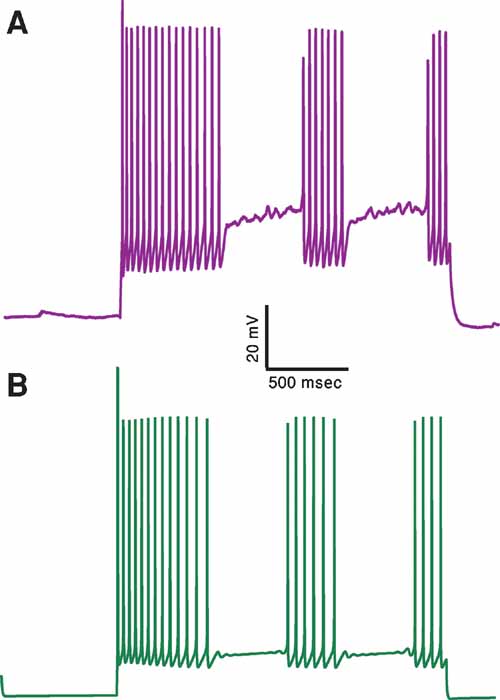
Figure 7. A proof of principle: generating an additional electrical class–stuttering neurons. (A) Experimental response of a stuttering interneuron to 2 seconds long, 150 pA depolarizing current (Markram et al., 2004). (B) Response of a model for this cell type to the same current input. A feature that measures the number of pauses in the firing response has been added to the other six features used before. This demonstrates that with this additional feature one can obtain a qualitative fit of the stuttering electrical class. The values of the channel conductances (in mS/cm²) obtained in this fit are: Na_t = 479; Na_p = 0; K_fast = 482; K_slow = 477; I_A = 99; Kv3.1 = 514; Ca = 6.57; SK = 85.4; I_h = 0; I_m = 2.36; Leak_soma = 0.00684; Leak_dendrite = 0.015.

Conflict of Interest Statement

The authors declare that the research was conducted in the absence of any commercial or financial relationships that should be construed as a potential conflict of interest.

Acknowledgements

We would like to thank Yael Bitterman for valuable discussions; Maria Toledo-Rodriguez for the experimental data and discussions regarding features; Phil Goodman for discussions regarding the selection of features; Srikanth Ramaswamy and Rajnish Ranjan for assistance with the literature on ion channels; Sean Hill for discussions regarding the manuscript. We also thank the two referees whose comments and suggestions helped to improve this manuscript significantly.

References

Achard, P., and De Schutter, E. (2006). Complex parameter landscape for a complex neuron model. PLoS Comput. Biol. 2, e94.

CrossRef Full Text

Adiga, N. R. et al. (2002). An overview of the BlueGene/L Supercomputer. Paper presented at: Supercomputing, ACM/IEEE 2002 Conference.

Bekkers, J. M. (2000a). Distribution and activation of voltage-gated potassium channels in cell-attached and outside-out patches from large layer 5 cortical pyramidal neurons of the rat. J. Physiol. 525, Pt 3 611–620.

Pubmed Abstract | Pubmed Full Text

Bekkers, J. M. (2000b). Properties of voltage-gated potassium currents in nucleated patches from large layer 5 cortical pyramidal neurons of the rat. J. Physiol. 525, 593–609.

CrossRef Full Text

Bibbig, A., Faulkner, H. J., Whittington, M. A., and Traub, R. D. (2001). Self-organized synaptic plasticity contributes to the shaping of gamma and beta oscillations in vitro. J. Neurosci. 21, 9053–9067.

Pubmed Abstract | Pubmed Full Text

Brette, R., Rudolph, M., Carnevale, T., Hines, M., Beeman, D., Bower, J.M., Diesmann, M., Morrison, A., Goodman, P.H., Harris, F.C., and Jr. (2007) Simulation of networks of spiking neurons: review of tools and strategies. J. Comput. Neurosci.

Pubmed Abstract | Pubmed Full Text

Carnevale, N. T., and Hines, M. L. (2005). The NEURON book (Cambridge, New York, Cambridge University Press).

Cohon, J. L. (1985). Multicriteria programming: Brief review and application. In Design Optimization, J. S. Gero, ed. (New York, NY, Academic Press).

De Schutter, E., and Bower, J. M. (1994). An active membrane model of the cerebellar Purkinje cell. I. Simulation of current clamps in slice. J. Neurophysiol. 71, 375–400.

Pubmed Abstract | Pubmed Full Text

Deb, K. (2001). Multi-objective optimization using evolutionary algorithms, 1st edn (Chichester, New York, John Wiley & Sons).

Deb, K., and Agarawal, R. B. (1995) Simulated binary crossover for continuous search space. Complex Syst. 9, 115–148.

Deb, K., Pratap, A., Agarwal, S., and Meyarivan, T. (2002). A fast and elitist multiobjective genetic algorithm: NSGA-II. IEEE Trans. evolutionary Comput. 6, 182–197.

CrossRef Full Text

Goldberg, D. E., and Richarson, J. (1987) Genetic algorithms with sharing for multimodal function optimization. In Proceedings of the First International Conference on Genetic Algorithms and Their Applications, pp. 41–49.

Goldman, M. S., Golowasch, J., Marder, E., and Abbott, L. F. (2001). Global structure, robustness, and modulation of neuronal models. J. Neurosci. 21, 5229–5238.

Pubmed Abstract | Pubmed Full Text

Golowasch, J., Goldman, M. S., Abbott, L. F., and Marder, E. (2002). Failure of averaging in the construction of a conductance-based neuron model. J. Neurophysiol. 87, 1129–1131.

Pubmed Abstract | Pubmed Full Text

Hamill, O. P., Huguenard, J. R., and Prince, D. A. (1991). Patch-clamp studies of voltage-gated currents in identified neurons of the rat cerebral cortex. Cereb. Cortex 1, 48–61.

Pubmed Abstract | Pubmed Full Text | CrossRef Full Text

Herz, A. V., Gollisch, T., Machens, C. K., and Jaeger, D. (2006). Modeling single-neuron dynamics and computations: A balance of detail and abstraction. Science 314, 80–85.

Pubmed Abstract | Pubmed Full Text | CrossRef Full Text

Hille, B. (2001). Ion channels of excitable membranes, 3rd edn (Sunderland, MA, Sinauer).

Pubmed Abstract | Pubmed Full Text

Hwang, C. L., and Masud, A. S. M. (1979). Multiple objective decision making, methods and applications: a state-of-the-art survey (Berlin, New York, Springer-Verlag).

Keren, N., Peled, N., and Korngreen, A. (2005). Constraining compartmental models using multiple voltage recordings and genetic algorithms. J. Neurophysiol. 94, 3730–3742.

Pubmed Abstract | Pubmed Full Text | CrossRef Full Text

Kirkpatrick, S., Gelatt, C. D., and Vecchi, M. P. (1983). Optimization by simulated annealing. Science 220, 671–680.

Pubmed Abstract | Pubmed Full Text

Koch, C., and Segev, I. (1998). Methods in neuronal modeling: from ions to networks, 2nd edn (Cambridge, MA, MIT Press).

Kohler, M., Hirschberg, B., Bond, C. T., Kinzie, J. M., Marrion, N. V., Maylie, J., and Adelman, J. P. (1996). Small-conductance, calcium-activated potassium channels from mammalian brain. Science 273, 1709–1714.

Pubmed Abstract | Pubmed Full Text ][CrossRef Full Text

Kole, M. H., Hallermann, S., and Stuart, G. J. (2006). Single Ih channels in pyramidal neuron dendrites: properties, distribution, and impact on action potential output. J. Neurosci. 26, 1677–1687.

Pubmed Abstract ][Pubmed Full Text | CrossRef Full Text

Korngreen, A., and Sakmann, B. (2000). Voltage-gated K+ channels in layer 5 neocortical pyramidal neurones from young rats: subtypes and gradients. J. Physiol. 525, 621–639.

CrossRef Full Text

LeMasson, G., and Maex, R. (2001) Introduction to equation solving and parameter fitting. In Computational Neuroscience,, E. De Schutter, ed. (Boca Raton, FL, CRC Press), pp. 1–24.

London, M., and Hausser, M. (2005). Dendritic computation. Annu. Rev. Neurosci. 28, 503–532.

Pubmed Abstract ][Pubmed Full Text ][CrossRef Full Text

MacLean, J. N., Zhang, Y., Johnson, B. R., and Harris-Warrick, R. M. (2003). Activity-independent homeostasis in rhythmically active neurons. Neuron 37, 109–120.

Pubmed Abstract ][Pubmed Full Text | CrossRef Full Text

Magistretti, J., and Alonso, A. (1999). Biophysical properties and slow voltage-dependent inactivation of a sustained sodium current in entorhinal cortex layer-II principal neurons: a whole-cell and single-channel study. J. Gen. Physiol. 114, 491–509.

Pubmed Abstract | Pubmed Full Text ][CrossRef Full Text

Mainen, Z. F., Joerges, J., Huguenard, J. R., and Sejnowski, T. J. (1995). A model of spike initiation in neocortical pyramidal neurons. Neuron 15, 1427–1439.

Pubmed Abstract | Pubmed Full Text | CrossRef Full Text

Mainen, Z. F., and Sejnowski, T. J. (1995). Reliability of spike timing in neocortical neurons. Science 268, 1503–1506.

Pubmed Abstract | Pubmed Full Text

Marder, E., and Goaillard, J. M. (2006). Variability, compensation and homeostasis in neuron and network function. Nat. Rev. Neurosci. 7, 563–574.

Pubmed Abstract ][Pubmed Full Text | CrossRef Full Text

Markram, H., Toledo-Rodriguez, M., Wang, Y., Gupta, A., Silberberg, G., and Wu, C. (2004). Interneurons of the neocortical inhibitory system. Nat. Rev. Neurosci. 5, 793–807.

Pubmed Abstract | Pubmed Full Text | CrossRef Full Text

Michalewicz, Z. (1992). Genetic algorithms + data structures = evolution programs (Berlin, New York, Springer-Verlag).

Mitchell, M. (1998). An introduction to genetic algorithms (Cambridge, MA, MIT Press).

Nowak, L. G., Sanchez-Vives, M. V., and McCormick, D. A. (1997). Influence of low and high frequency inputs on spike timing in visual cortical neurons. Cereb. Cortex 7, 487–501.

Pubmed Abstract | Pubmed Full Text | CrossRef Full Text

Press, W. H. (2002). Numerical recipes in C : the art of scientific computing, 2nd edn (Cambridge Cambridgeshire, New York, Cambridge University Press).

Prinz, A. A., Abbott, L. F., and Marder, E. (2004a). The dynamic clamp comes of age. Trends Neurosci. 27, 218–224.

CrossRef Full Text

Prinz, A. A., Billimoria, C. P., and Marder, E. (2003). Alternative to hand-tuning conductance-based models: construction and analysis of databases of model neurons. J. Neurophysiol. 90, 3998–4015.

Pubmed Abstract | Pubmed Full Text | CrossRef Full Text

Prinz, A. A., Bucher, D., and Marder, E. (2004b). Similar network activity from disparate circuit parameters. Nat. Neurosci. 7, 1345–1352.

CrossRef Full Text

Rapp, M., Yarom, Y., and Segev, I. (1996). Modeling back propagating action potential in weakly excitable dendrites of neocortical pyramidal cells. Proc. Natl. Acad Sci. USA 93, 11985–11990.

CrossRef Full Text

Reuveni, I., Friedman, A., Amitai, Y., and Gutnick, M. J. (1993). Stepwise repolarization from Ca2+ plateaus in neocortical pyramidal cells: evidence for nonhomogeneous distribution of HVA Ca2+ channels in dendrites. J. Neurosci. 13, 4609–4621.

Pubmed Abstract | Pubmed Full Text

Rudy, B., and McBain, C. J. (2001). Kv3 channels: voltage-gated K+ channels designed for high-frequency repetitive firing. Trends Neurosci. 24, 517–526.

Pubmed Abstract | Pubmed Full Text ][CrossRef Full Text

Schneidman, E., Freedman, B., and Segev, I. (1998). Ion channel stochasticity may be critical in determining the reliability and precision of spike timing. Neural Comput. 10, 1679–1703.

Pubmed Abstract | Pubmed Full Text | CrossRef Full Text

Schulz, D. J., Goaillard, J. M., and Marder, E. (2006). Variable channel expression in identified single and electrically coupled neurons in different animals. Nat. Neurosci. 9, 356–362.

Pubmed Abstract | Pubmed Full Text | CrossRef Full Text

Schulz, D. J., Goaillard, J. M., and Marder, E. E. (2007). Quantitative expression profiling of identified neurons reveals cell-specific constraints on highly variable levels of gene expression. Proc. Natl. Acad Sci. USA 104, 13187–13191.

Pubmed Abstract | Pubmed Full Text | CrossRef Full Text

Shen, G. Y., Chen, W. R., Midtgaard, J., Shepherd, G. M., and Hines, M. L. (1999) Computational analysis of action potential initiation in mitral cell soma and dendrites based on dual patch recordings. J. Neurophysiol. 82, 3006–3020.

Pubmed Abstract | Pubmed Full Text

Shinomoto, S., Shima, K., and Tanji, J. (2003). Differences in spiking patterns among cortical neurons. Neural Comput. 15, 2823–2842.

Pubmed Abstract | Pubmed Full Text | CrossRef Full Text

Taylor, A. L., Hickey, T. J., Prinz, A. A., and Marder, E. (2006). Structure and visualization of high-dimensional conductance spaces. J. Neurophysiol. 96, 891–905.

CrossRef Full Text

Pubmed Abstract | Pubmed Full Text

Traub, R. D., Contreras, D., Cunningham, M. O., Murray, H., LeBeau, F. E., Roopun, A., Bibbig, A., Wilent, W. B., Higley, M. J., and Whittington, M. A. (2005). Single-column thalamocortical network model exhibiting gamma oscillations, sleep spindles, and epileptogenic bursts. J. Neurophysiol. 93, 2194–2232.

Pubmed Abstract | Pubmed Full Text | CrossRef Full Text

Toledo-Rodriguez, M., Blumenfeld, B., Wu, C., Luo, J., Attali, B., Goodman, P., and Markram, H. (2004). Correlation maps allow neuronal electrical properties to be predicted from single-cell gene expression profiles in the rat neocortex. Cereb. Cortex 14, 1310–1327.

Pubmed Abstract | Pubmed Full Text | CrossRef Full Text

Vanier, M. C., and Bower, J. M. (1999). A comparative survey of automated parameter-search methods for compartmental neural models. J. Comput. Neurosci. 7, 149–171.

Pubmed Abstract | Pubmed Full Text | CrossRef Full Text

Victor, J. D., and Purpura, K. P. (1996). Nature and precision of temporal coding in visual cortex: a metric-space analysis. J. Neurophysiol. 76, 1310–1326.

Pubmed Abstract | Pubmed Full Text