Ensembles of gustatory cortical neurons anticipate and discriminate between tastants in a single lick
- 1 Department of Neurobiology, Duke University, Durham, NC, USA
- 2 Institute of Statistics and Decision Sciences, Durham, NC, USA
- 3 Department of Biomedical Engineering, Durham, NC, USA
- 4 Department of Psychological and Brain Sciences, Durham, NC, USA
- 5 Center for Neuroengineering, Duke University, Durham, NC, USA
- 6 Edmond and Lily Safra International Institute of Neuroscience of Natal, Natal RN, Brazil
- 7 Brain and Mind Institute, École Polytechnique Fédérale de Lausanne, Lausanne, Switzerland
The gustatory cortex (GC) processes chemosensory and somatosensory information and is involved in learning and anticipation. Previously we found that a subpopulation of GC neurons responded to tastants in a single lick (Stapleton et al., 2006 ). Here we extend this investigation to determine if small ensembles of GC neurons, obtained while rats received blocks of tastants on a fixed ratio schedule (FR5), can discriminate between tastants and their concentrations after a single 50 μL delivery. In the FR5 schedule subjects received tastants every fifth (reinforced) lick and the intervening licks were unreinforced. The ensemble firing patterns were analyzed with a Bayesian generalized linear model whose parameters included the firing rates and temporal patterns of the spike trains. We found that when both the temporal and rate parameters were included, 12 of 13 ensembles correctly identified single tastant deliveries. We also found that the activity during the unreinforced licks contained signals regarding the identity of the upcoming tastant, which suggests that GC neurons contain anticipatory information about the next tastant delivery. To support this finding we performed experiments in which tastant delivery was randomized within each block and found that the neural activity following the unreinforced licks did not predict the upcoming tastant. Collectively, these results suggest that after a single lick ensembles of GC neurons can discriminate between tastants, that they may utilize both temporal and rate information, and when the tastant delivery is repetitive ensembles contain information about the identity of the upcoming tastant delivery.
Introduction
The gustatory cortex (GC) is a nexus for converging streams of chemosensory (Accolla et al., 2007 ; Baylis and Rolls, 1991 ; Katz et al., 2001 , 2002 ; Miyaoka and Pritchard, 1996 ; Scott et al., 1991 ; Smith-Swintosky et al., 1991 ; Stapleton et al., 2006 ; Yamamoto et al., 1980 , 1988 , 1984 ; Yaxley et al., 1990 ), somatosensory (Cerf-Ducastel et al., 2001 ; De Araujo and Rolls, 2004 ; Katz et al., 2001 ; Ogawa and Wang, 2002 ; Stapleton et al., 2006 ; Verhagen et al., 2004 ; Yamamoto et al., 1988 ), and hedonic information (Fontanini and Katz, 2006 ; Sewards, 2004 ; Small et al., 2003 ; Yamamoto et al., 1989 ). In addition to processing sensory data, the GC is also involved in learning (Balleine and Dickinson, 2000 ; Bermudez-Rattoni et al., 2005 ), expectation and anticipation (Nitschke et al., 2006 ; Yamamoto et al., 1988 ), and attention (Fontanini and Katz, 2006 ).
The pioneering studies of Halpern and colleagues showed that trained rats can discriminate between tastants on the basis of a single lick (Halpern and Marowitz, 1973 ; Halpern and Tapper, 1971 ). Our previous work with freely licking rats demonstrated that single GC neurons could respond to tastants within the span of one lick (∼150 ms). We also found, as have others, that GC neurons were multimodal and broadly tuned (Katz et al., 2001 ; Ogawa and Wang, 2002 ; Smith-Swintosky et al., 1991 ; Stapleton et al., 2006 ). In contrast, most electrophysiological studies of GC neurons average the firing rates over 3–10 seconds and define chemosensory neurons as those whose evoked firing rates differ significantly from background firing levels (Miyaoka and Pritchard, 1996 ; Scott et al., 1991 ; Smith-Swintosky et al., 1991 ; Soares et al., 2007 ; Yamamoto et al., 1984 ; Yaxley et al., 1990 ). One potential issue with identifying chemosensory responses in this manner is that during such a long period of time (i.e. several seconds) somatosensory and hedonic signals may be conflated with the chemosensory information (Katz et al., 2001 ).
In the present experiments the firing patterns from simultaneously recorded GC neurons were analyzed with a Bayesian generalized linear model (GLM) (Dobson, 2002 ). This method of analysis offers several advantages over the traditional techniques of cluster analysis and multidimensional scaling (Miyaoka and Pritchard, 1996 ; Smith-Swintosky et al., 1991 ; Yaxley et al., 1990 ), both of which, in the context of gustatory processing, usually only consider firing rates and cannot readily accommodate multimodal neurons. In contrast, the GLM can employ rate information as well as temporal firing patterns, the latter of which is also important for gustatory coding (Di Lorenzo and Victor, 2003 ; Katz et al., 2001 ; Stapleton et al., 2006 ). Second, the GLM can quantify the effects of multiple variables such as tastant identity, trial number, and unreinforced licks on the spike trains (Stapleton et al., 2006 ). Third, the GLM can estimate the underlying distributions of the neural data (Dobson, 2002 ).
This study employed an FR5 schedule in which a block of trials consisted of eight deliveries of the same tastant. Therefore, it was possible for subjects within each block to predict the identity of the future tastant. Thus, the second goal of this study was to determine whether neural information during the unreinforced licks could predict the upcoming tastant.
Materials and Methods
Subjects
Male Long-Evans rats (n = 6) were purchased from Harlan Bioproducts for Science Inc. (Indianapolis, IN). Prior to surgery, all subjects weighed 300–450 g. The rats were housed separately in Plexiglas cages and were maintained on a 12 hour light/dark schedule, with experiments conducted during the light phase of the cycle. The subjects were allowed to recover from surgery for at least 2 weeks, after which they were placed on a 20 hour water deprivation schedule. In addition to the water available during each 2- or 3- hour test session, subjects were also given 1 hour of access to water in their home cages. Purina rat chow was available ad libitum.
All protocols were approved by the Duke University Institutional Animal Care and Use Committee.
Surgery
The details of this surgery are given elsewhere (Katz et al., 2001 ; Soares et al., 2007 ; Stapleton et al., 2006 ). Briefly, rats were first anesthetized with a 5% halothane/air mix and then with a 50 mg/kg IP injection of sodium pentobarbital. Moveable electrode bundles (16 15 μm tungsten microwires per cannula shaft) were implanted bilaterally above GC (1.3 mm anterior, 5.2 mm lateral, and 4.7 mm horizontal from bregma) (Kosar et al., 1986 ; Stapleton et al., 2006 ), and dental acrylic was applied to seal the skull and electrode bundles. Following 1–2 weeks of recovery, the electrodes were lowered 250 μm per day until reaching the GC.
General Electrophysiology
Recording commenced after the electrodes had penetrated GC. The electrodes were lowered further in 125 μm increments and a new ensemble was obtained when the signals at the current location had degraded.
Neural activity was recorded continuously during the experiment. Differential recordings were sent to a parallel processor that digitized the analog signals from multiple channels at 40 kHz (Plexon, Dallas, TX). Discriminable action potentials with a signal/noise ratio ≥ 3:1 were isolated online from each channel through the use of template matching in conjunction with 3-D principal component analysis (PCA) (Katz et al., 2001 ; Nicolelis et al., 2003 ; Soares et al., 2007 ; Stapleton et al., 2006 ). The refractory period for single units was fixed at 2 ms. Time-stamped records of stimulus onsets, spiking events, and all spike waveforms were stored digitally for additional offline sorting.
For the FR5 experiment, a total of 178 neurons were obtained from four rats. The first subject yielded 39, the second yielded 50, and the third and fourth rats yielded 40 and 49 neurons, respectively. The average number of neurons per wire was 1.4. For the random FR5 experiment, 18 neurons were collected from two animals.
Behavioral Apparatus
All testing occurred in Med Associates (St. Albans, VT) operant chambers that were housed within sound attenuating boxes. Recessed at the end of the operant chamber was a lick tube that comprised 12 20-gauge stainless steel tubes housed in a larger steel tube (id = 7.5 mm). Positioned in front of the lick tube was an infrared Med Associates lickometer. Taste solutions were contained in 50 mL chromatography columns located outside of the sound attenuating boxes (Kontes Flex-Columns, Fisher Scientific, Hampton, NH), and the columns were maintained under ∼8 psi of air or nitrogen, thus ensuring that a constant volume of tastant was delivered. Computer-controlled solenoids (Parker Hannifin Corporation, Fairfield, NJ), also located outside of the sound attenuating boxes, regulated tastant delivery. Within 10 ms after a lick was detected due to the breaking of the infrared beam, one of the valves opened and delivered 50 μL of fluid.
Behavioral Testing
Water-deprived rats were tested on a fixed ratio schedule (FR5). In a given testing session subjects were presented with a set of taste solutions. These included sucrose (0.025, 0.075, 0.1, and 0.3 M), monosodium glutamate (MSG) (0.025, 0.075, 0.1, and 0.3 M), and NaCl (0.025, 0.075, 0.1, and 0.3 M); quinine HCl (0.0001 and 0.0003 M); citric acid (0.005 and 0.01 M); and distilled water. All chemicals were obtained from Sigma–Aldrich (St. Louis, MO) and were reagent-grade.
Under the fixed ratio schedule (FR5) water-deprived rats were trained to drink from the lick tube such that 50 μL of a given tastant was delivered every fifth lick (i.e., the previous four licks were “dry” in that no fluid was delivered). Reinforced licks were defined as those in which a tastant was delivered, and unreinforced licks were those in which tastants were not delivered. A block consisted of eight deliveries (trials) of a particular tastant, after which the block ended and a 5–10 second interblock interval (IBI) began. At the end of the IBI, one or two water “washouts” were delivered (50–100 μL). The washout was followed by a second 5–10 second IBI, and then another tastant block began. The tastant delivered across blocks was randomized without replacement using a Latin square protocol. Within a test session, each tastant was presented in multiple blocks (3–8) for a total of 24–64 deliveries, and during each experiment subjects regularly consumed 25–35 mL of fluid. Initially subjects consumed all fluids equally rapidly and completed each block within about 8–10 seconds. As the experiment progressed, however, subjects still consumed palatable stimuli such as sucrose at the same rate (8–10 seconds per block) but decreased their drinking rates for less palatable stimuli such as quinine. The subjects frequently required more than 20 minutes to complete a block of quinine trials. Recordings ceased when the subjects did not emit a lick response for more than 45 minutes.
To prevent the subjects from predicting the upcoming tastant delivery, a second set of control experiments were conducted in which the tastant delivered on the fifth lick was chosen at random and without replacement. This experiment was termed “random FR5.” In this protocol a block consisted of eight deliveries of different tastants, and blocks were separated by an IBI, a water washout, and a second IBI.
Data Modeling
In recordings from the GC we found that chemosensory activity occurs in 150 ms (Stapleton et al., 2006 ), which is the average duration of a single lick (Gutierrez et al., 2006 ; Wiesenfeld et al., 1977 ). Chemosensory neurons were defined as those that discriminated between reinforced and unreinforced licks and between tastants (Stapleton et al., 2006 ). Non-chemosensory neurons were those that did not meet both of these requirements. Here we analyze the ensemble response properties of these previously collected neurons, of which there were 61 identified as chemosensory and 117 that were defined as non-chemosensory.
As before, 150 ms windows were taken from the third, unreinforced lick and from the fifth, reinforced lick. The third unreinforced lick was chosen for the analysis to prevent any potential overlap with the time window for the reinforced lick as some licks are a little shorter than 150 ms. As justified previously, for each neuron within a given ensemble, spikes that fell within the 150 ms window were then binned in 15 ms increments (Stapleton et al., 2006 ). After the binning the data, for the reinforced licks the spike counts corresponding to the third and seventh trials for each block of eight were dropped from the data set. This is equivalent to dropping 25% of the data. For each block of the unreinforced lick data the first, third, and seventh trials (or 37.5% of the trials) were dropped (see below for justification). The remaining data for each ensemble were analyzed with a Bayesian GLM (Dobson, 2002 ), and the reserved data from each ensemble were later used for prediction purposes. Each ensemble was analyzed separately, and separate models were constructed for the reinforced and unreinforced lick data for each ensemble.
The model was defined as follows: Let Yijkl be the number of spikes for neuron i, tastant j, trial k, and time bin l. Define Wijk ≡ Σl Yijkl, where Wijk is the number of spikes for neuron i, tastant j, and trial k in the entire 150 ms window.
The following statistical model for the Ws and Ys was adopted. Let Yijkl ∼ Poi(λijkl), where the parameter lambda represents the Poisson distribution of the number of spikes in a 15 ms bin that, in turn, depends on the neuron, tastant, trial, and bin. It is assumed that the Yijkls are mutually independent (given the λijkls) and therefore that Wijk ∼ Poi(λijk), where λijk = Σl λijkl and the Wijks are mutually independent.
In this model ln(λijk) = cij + dijk, where exp(cij) represents the mean firing rate – in spikes per 150 ms – of neuron i to tastant j; dijk is an adjustment parameter that is expected to be small because firing rates change slightly over time and therefore from trial to trial. For the ith neuron, the variability of the cijs as j ranges over all tastants captures how that neuron changes its firing rate in response to different tastants. λijk represents the rate parameter of the model.
It follows that each spike in a 150 ms window must fall into one of ten 15 ms bins. The probability of falling in the l’th bin is λijkl/λijk. More generally, one may write
where aijkl = λijkl/λijk aijkl represents the temporal parameter of the model.
This model was implemented in OpenBugs (www.mrc-bsu.cam.ac.uk/bugs ) with priors
 with separate means μj for each neuron and a precision of
  , where μj ∼ Norm(0, 106) and where σ1 ∼ U (0, 10), and
  , with mean 0 and precision
  , where σ2 = σ1 * w, and w ∼ U (0, 100). The terms cij and dijk were both censored for values below -5. The prior for aijkl was constructed such that

After the model had been compiled and the appropriate initial values had been loaded, BUGS used a Gibbs sampler to find the posterior distributions of all unknown parameters. A total of 40 000 iterations were conducted, and the first 1000 samples were discarded, although we found that the model always converged well before the first 1000 iterations. Hence, 39 000 iterations remained, and the data were then thinned in increments of 100 to make the analysis more computationally tractable. This resulted in a final set of 390 iterations from which to construct the posterior distributions for these terms.
Data Prediction
When the model had run to completion, the data for aijkl, cij, and σ2 were imported into R (www.R-project.org
). To reconstruct the overall fluctuations in firing rate across the tastant deliveries, 390 values of d were randomly drawn from N(0, σ2) where σ2 is a vector of corresponding length. Then, the distribution of the spike sums,  is
is
for h as the iteration number (1, …, 390). The distributions of the ensemble firing patterns for the different tastants,  , across all trials is then

Three models were then constructed to determine how rate and temporal information contribute to tastant discrimination. The three model types are described below.
Combined model. In this model is a function of both  , the rate parameter, and
  , the temporal parameter. Because the following model is a function of (and hence of both parameters), it is referred to as the combined model. Let the withheld data for a given ensemble and for a given tastant be denoted as Xijkl. Then, the probability of observing X given that a single delivery of a particular tastant Tj has occurred is
For each tastant the probability P(Xijkl|Tj) is calculated, and the subscript k denotes the particular observed trial. The tastant that is predicted to have occurred given the ensemble firing pattern on the particular trial is the one for which P(Xijkl|Tj) is the greatest. These calculations are then repeated for each delivery of X. The number of times that the true tastant was predicted correctly was then divided by the total number of observations of that particular tastant to determine the percentage of correct guesses for that ensemble.
Each ensemble (n = 13) was analyzed individually, and ensembles ranged in size from 7 to 27 neurons. For ensembles in which 12 tastants were delivered (n = 6), the odds of correctly identifying the tastant delivery by chance were 1 in 12, or about 8.3%. For ensembles tested with seven (n = 2) or eight (n = 4) stimuli, the odds of correctly identifying tastants by chance were either 1 in 7 (∼14.3%) or 1 in 8 (12.5%), respectively. One ensemble was tested with five tastants, and the odds were then 1 in 5, or 20%.
Rate model. Analyses were also performed with the distributions of the spike sums () to determine how well firing rates alone could predict tastant identity. In this case, we let Zijk ≡ Σl Xijkl, where Zijk is the total number of observed spikes in the 150 ms window. Then, the predictions are given by
If the first model correctly identifies more tastants than the second model, then a combination of temporal coding and rate coding contains more information than rate coding alone.
Temporal model. Similar analyses were conducted with the distributions of the values of to determine if a temporal profile would be sufficient to predict tastant identity. The values of a sum to one across the time bins, so a essentially reflects how the spikes are distributed in the bins and not the actual spike counts in each bin per se. In this case,

Hence, predictions from the temporal model can be compared to the rate model and to the combined model to determine which sort of code most faithfully represents taste stimuli.
To quantify the ability of the combined model to predict tastants across the ensembles, several summary analyses were performed. First, to determine if all of the ensembles collectively could predict tastants above chance, the total number of correct predictions for all tastants across all 13 ensembles was summed together. Then, the total number of observations withheld from all of the ensembles was summed together. To determine the percent of total deliveries correctly predicted by the model, the total number of correct predictions was divided by the total number of observations, and this quantity was multiplied by 100. Chance prediction levels were constructed by multiplying the individual chance level for each ensemble (i.e., 8.3% for ensembles with 12 tastants) by the total number of observed trials for that ensemble. The products for each ensemble were then summed and this sum was divided by the total number of observations and then multiplied by 100. This quantity is a weighted average of the chance level given the number of observations of each ensemble and the number of tastants tested for each ensemble. If the ensemble prediction level for the combined model is greater than the weighted chance level, then the ensembles collectively can discriminate gustatory stimuli. The chance cutoff level is analogous to an alpha level of 0.05. Hence, anything greater than chance is considered to be statistically significant. Similar calculations were performed for the rate and temporal models, and the percentages of correct identifications were compared to chance. If for either model the percentage of correct guesses was above chance, then that particular model could predict taste stimuli. Likewise, the models were also ranked against each other according to how well each predicted the tastants. Because these models are Bayesian, and because each possesses a large number of parameters, it is standard practice to compare such models simply in terms of the percentage of data that each can predict. It should also be noted that previous tests revealed that including temporal information resulted in a much better fit of the spike trains in comparison to analyzing rate information alone (Stapleton et al., 2006 ).
The predictions were also considered in terms of how well the individual taste stimuli were identified. In this case, the total number of times each tastant and concentration were correctly identified across all ensembles was divided by the total number of observations for that stimulus. The chance levels were calculated for each stimulus separately given the number of tastants tested in each ensemble and the total number of observations for each tastant. The percentage of correct identifications was compared to the weighted chance value to determine if the ensembles could discriminate that particular taste stimulus above chance, and these analyses were conducted for all three models.
It is to be expected that the firing patterns corresponding to concentrations of the same tastant are more similar to each other than they are to firing patterns of a perceptually different tastant (Ganchrow and Erickson, 1970 ; Stopfer et al., 2003 ). Hence, if the models could not correctly identify exactly which concentration of a particular stimulus was delivered, the models might suggest that a different concentration had been presented instead of incorrectly classifying the patterns as corresponding to a different tastant. In this case, regardless of concentration, the total number of correct tastant classifications (i.e., MSG, NaCl, etc.), was divided by the total number of observations of that tastant across all concentrations. The values for chance were determined for each ensemble by counting the number of concentrations of each tastant and dividing that by the number of tastants tested in that ensemble. The chance levels were multiplied by the total number of observations in each ensemble for each tastant type. These values were then divided by the total number of observations across all ensembles. The tastant prediction rates were compared to the chance levels to determine whether the particular model could correctly classify the tastant type. The prediction levels for each model were compared to determine which model best classified each stimulus. To determine which model exhibited the best performance, the total numbers of correct classifications were summed across ensembles and this value was divided by the total number of observations for all stimuli and then converted to a percentage (see Figures 6 , 7 , and 11 ). This percentage was compared to the chance level to determine the extent to which each model could classify tastants overall.
In the first set of analyses, the model was employed to discriminate between the different tastants and their concentrations, which was a total of 17 stimuli. In the second set of analyses, the model was used to classify tastants into types, and this corresponded to a total of six categories. As the number of stimuli increases, the chance level decreases, and the prediction levels also decrease. To demonstrate that the model was indeed capable of discriminating between stimuli at high level of precision, the model was also tested with just two stimuli (i.e., 0.3 M MSG and 0.3 M NaCl, etc.) from the first ensemble for each rat. The first ensemble from each animal was chosen because this ensemble usually had the highest prediction rates when all tastants and their concentrations were tested (see below).
The analyses described above pertain to those trials conducted on the reinforced lick data. To determine whether ensembles of neurons could predict the identity of future tastants, a second set of similar analyses were conducted on the unreinforced lick data. If anticipatory information was present in the unreinforced lick activity, then the spike trains should be able to discriminate between tastants. If anticipatory activity is not present, however, then the odds of correctly identifying the tastants should be at chance. For the unreinforced lick data, trials one, three, and seven were dropped from each block and then the combined, rate, and temporal models were constructed with the remaining data. Predictions with trials three and seven were conducted as outlined above. As a control, the first unreinforced lick trial at the start of each tastant block in the FR5 schedule was also used for prediction purposes. Because tastant delivery was randomized across blocks, it is expected that the rats should not be able to predict which tastant would be delivered at the start of the block. Hence, we expect that the data for first unreinforced lick should be unable to predict the upcoming tastant.
Two additional experiments were conducted in which the delivery of the tastants was randomized within each block (random FR5 schedule). In this case, we would expect that the spike trains during the reinforced licks should still contain information about the tastant delivered. In contrast, the unreinforced lick data should not be predictive because the subjects should be unable to anticipate the identity of the future tastants. The reinforced lick data from the random FR5 experiment were analyzed in the same manner as the previous data described above. Only trials three and seven were dropped from the unreinforced data for the random FR5 experiment, as the comparison with trial one was unnecessary.
One possibility is that the unreinforced lick data from the first set of experiments actually contain residual information from the previous tastant delivered. If this is the case, then the spike trains corresponding to the unreinforced licks in the random FR5 schedule might actually predict the previous tastant delivered. To test for this, trial licks three and seven were dropped from the data set and the remaining spike trains were modeled with respect to the previous tastant. If there is no residual activity from the previous tastant, then the predictions should be at or below chance.
Neuron dropping. To determine how the number of neurons in an ensemble affects prediction strength, a neuron-dropping analysis was performed. In this analysis, the data for a given neuron were dropped from the ensemble and the predictions were then conducted. The data for the neuron were then reinserted into the ensemble and a second neuron was dropped, etc. In this manner, the predictions were conducted in the absence of each neuron, and then all the prediction probabilities following each drop were averaged. Then, all possible combinations of two neurons were dropped from the ensemble, and the predictions were conducted again with the remaining sets of data. This process was continued in a combinatorial manner until all possible combinations of neuron numbers had been dropped from the data set. Because of computational constraints, three representative ensembles from different subjects were analyzed.
Histology
Following completion of the experiments, the rats were deeply anesthetized with an intraperitoneal injection of Nembutal (150 mg/kg) and perfused transcardially with 120 cc of PBS followed by 120 cc of formalin (10%). Brains were removed and stored in a sucrose/formalin solution (30% sucrose w/v) for 24 hours of postfixation. The tissue was sectioned through GC in 50 μm coronal slices and stained with cresyl violet to visualize cell bodies. This is sufficient to visualize electrode tracks, which were subsequently mapped to verify placement. It was found that the electrodes generally spanned from layers II to VI, and the electrodes were located primarily in the dysgranular insular cortex (Soares et al., 2007 ; Stapleton et al., 2006 ).
Results
Previously, we found that a subpopulation of single GC neurons (n = 178) were broadly tuned and responded to tastants in the span of 150 ms (Stapleton et al., 2006 ). Using this same data set and a second data set of neurons (n = 18) tested on the random FR5 schedule we extend the findings of our previous study and show that small ensembles of GC neurons can discriminate between tastants and their concentrations. Of the 178 neurons from the first data set 61 were classified as chemosensory as were 11 of the 18 neurons in the second data set. Our current results are divided into five sections. The first illustrates the response properties of single GC units obtained during the FR5 and random FR5 test schedules. The second presents a general summary of the prediction strengths for the ensembles during the reinforced and unreinforced licks. In the third, predictions during the reinforced licks are explored as a function of individual tastant and concentration as well as general tastant classification. The fourth explores how single units contribute information to the ensemble prediction, and the fifth and final section provides evidence of tastant anticipation during the unreinforced licks.
Single Unit Response Properties
Figure 1 depicts the responses of two GC neurons to a set of five taste stimuli. The neuron depicted in Figure 1 A was tested on the FR5 schedule, and the neuron presented in Figure 1 B was tested with the random FR5 schedule. The upper part of each graph depicts the raster plots, in which the spike train corresponding to the first tastant delivery occurs at the top of the plot. The average activity across all of the deliveries of a particular tastant is depicted in the peristimulus time histograms (PSTHs) located below the raster plots. In these panels a given tastant was delivered at 0 ms (red triangles aligned at 0 ms). For most trials, the two unreinforced lick times before and after tastant delivery occurred at about ±150 ms and are denoted by the red inverted triangles overlaid on the raster plots. It is seen that after tastant delivery both neurons exhibit rapid increases in firing rate. We previously reported that in the majority of chemosensory neurons such activity decays before the onset of the next unreinforced lick (Stapleton et al., 2006 ). It is seen that both of these neurons are broadly tuned, but upon inspection of the PSTHs it is clear that the timing of the spikes is different according to the tastant delivered. In Figure 1 A, it is evident that the response patterns for 0.1 M NaCl are different than those for 0.1 M sucrose and in Figure 1 B, the responses of these two stimuli differ in both amplitude and duration. This shows that chemosensory responses can differ in their firing rates and temporal patterns.
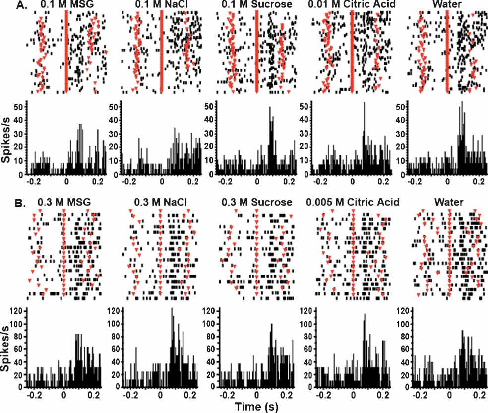
Figure 1. GC neurons respond rapidly to tastants under the FR5 and random FR5 schedules. (A) These peristimulus time histograms (PSTHs) represent the activity of a single neuron tested on the FR5 schedule. Each panel depicts the neuron's response to one concentration of a particular tastant. The raster plots are depicted at the top of each panel, and the top row represents the first stimulus trial. The bottom portion of each panel depicts the corresponding PSTH. Zero on the abscissa denotes the time of tastant delivery (red triangles aligned at 0 ms on the raster plots), and the ordinate is given in terms of spikes per second. The unreinforced lick times are depicted as inverted triangles overlaid on the raster plots at approximately ±150 ms. The bin size for the PSTHs is 5 ms. The activity of this neuron indicates that it is broadly tuned and responds to all of the tastants. Note that the pattern of its responses is different for different tastants. (B) These PSTHs depict the activity of a single neuron tested on the random FR5 schedule. Conventions are the same as in A. As with the neuron depicted above, this neuron is also broadly tuned and responds to all proffered tastants. NaCl and citric acid evoked the greatest responses from this unit.
As described in the Methods section, the firing patterns of each neuron in an ensemble can be partitioned into rate and temporal components. Figure 2 illustrates how this was achieved for two different neurons. Each panel depicts the average proportion of spikes in each bin for a particular tastant (solid line), and the 10 and 90% quantiles are shown as the dotted lines. As seen in Figure 2 A, it is clear that for this neuron the temporal patterns are very different for the different tastants. For this neuron the firing rates ranged between a minimum of 8.8 spikes/seconds and a maximum of 18.8 spikes/seconds for 0.075 M MSG and 0.1 M sucrose, respectively. Note that the average firing rates for all NaCl concentrations are the same but that the concentrations elicited different temporal patterns. Note also, for example, that 0.3 M NaCl evoked the greatest response in bin 7, which corresponds to 105 ms, while 0.1 M NaCl evoked a peak response in bin 8, or 120 ms. These two temporal patterns are significantly different because there is little overlap between the peak response times for these particular taste stimuli. For 0.3 and 0.1 M sucrose, however, the firing rates alone are sufficient to discriminate between the stimuli. In this case, the average firing rate ± SEM for 0.3 M sucrose is 13.6 ± 3.6 spikes/seconds, while the firing rate for 0.1 M sucrose is 18.8 ± 4.9 spikes/seconds. Here, there is no significant difference between the temporal profiles for these two stimuli because there is considerable overlap between their respective quantiles.
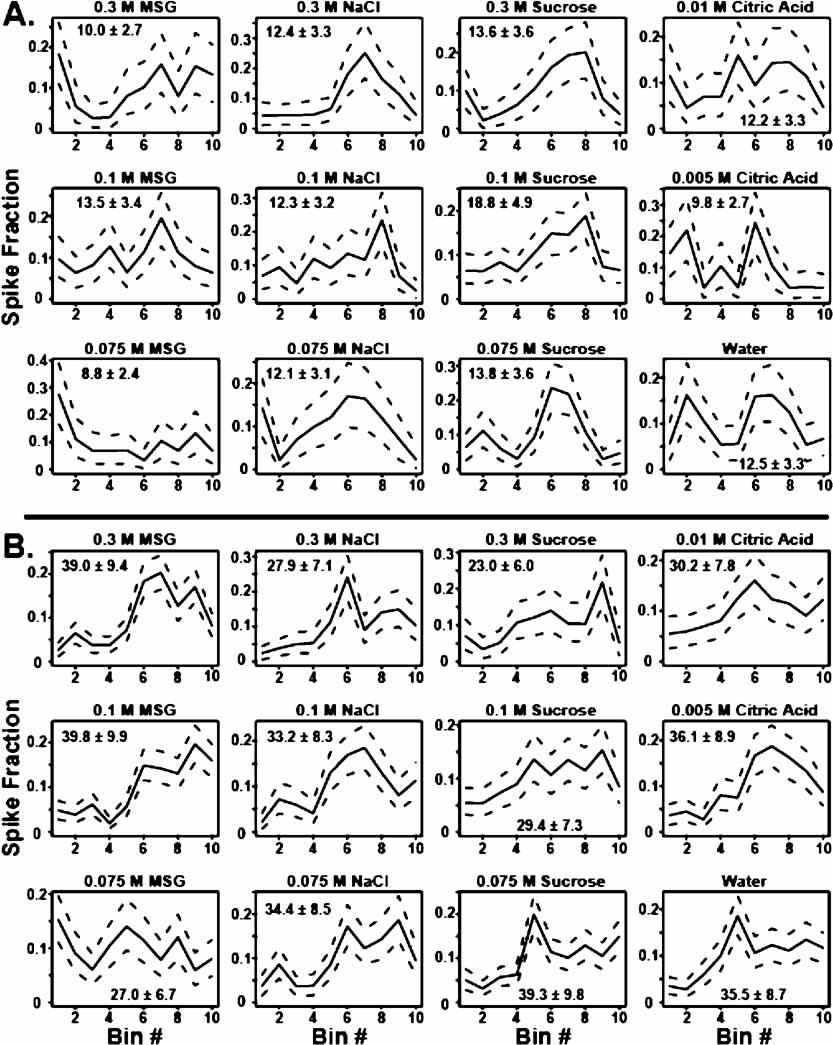
Figure 2. Partitioning single neuron firing patterns into rate and temporal components. (A) This set of 12 panels depicts the way in which the firing patterns of a single unit were decomposed into temporal and rate components. Each graph represents the neuron's temporal response to one concentration of a particular tastant. The abscissa corresponds to the bin number within the 150 ms window following tastant delivery. Each bin represents 15 ms. The fraction of spikes that fall into each bin is given on the ordinate. The average proportion of spikes that fall in each bin is depicted as the solid black line, and 10th and 90th quantiles for the averages are shown as the dashed lines. The average firing rates (spikes/seconds) and SEMs for each tastant are also presented. The temporal patterns for the 0.1 and 0.3 M sucrose exhibit substantial overlap and therefore are not significantly different, but the average firing rates do differ significantly. For 0.1 and 0.3 M NaCl, the temporal patterns differ substantially in their peak response times, but the firing rates for these stimuli are not significantly different. (B) In the case of 0.075 and 0.3 M MSG, both the temporal profiles and the firing rates for this neuron are significantly different. In contrast, note that firing rates for 0.1 M MSG and 0.075 M sucrose are the same but that the associated temporal profiles are very different.
Figure 2 B depicts the responses of a second chemosensory neuron to the same set of tastants. In this neuron the firing rates ranged between 23 spikes/seconds for 0.3 M sucrose and 39 spikes/seconds for both 0.075 M sucrose and 0.1 M MSG. Note that for these two sucrose concentrations both the rate and the temporal patterns are different. Indeed this is frequently the case as illustrated by this neuron's different temporal and firing rate responses to 0.3 and 0.075 M MSG. Because both rate and temporal information can be used to discriminate between these two stimuli, coding mechanisms that use both types of information (combined) may be better than coding schemes using only one parameter (temporal patterns or average firing rates) although in many cases, as we will show below, the types of information may be redundant.
On the basis of the partitioning of information into rate and temporal components we then determined whether either of the individual models or the combined model better predicted concentrations of tastants in a single trial.
General Ensemble Predictions
Figure 3 B depicts the overall ensemble prediction levels for the reinforced and unreinforced licks for subjects on the FR5 protocol (n = 17 taste stimuli). The model type is displayed on the abscissa, and the percentage of correct tastant classifications is presented on the ordinate. The total prediction levels for the reinforced licks are presented in Figure 3 A. The combined model is depicted in red, while the predictions for the rate model and the temporal model alone are presented in blue and green, respectively. The chance prediction rate is shown in black. While all three models predict tastants above chance, the combined model correctly identified the most tastant deliveries (17.6%). For the combined model, following the reinforced licks, 12 of 13 ensembles were capable of predicting tastants based on the spike trains. When only rate codes were considered, 10 of 13 ensembles predicted tastants above chance, and when only temporal patterns were considered, 11 of 13 ensembles predicted tastants above chance. The rate and temporal models correctly identified the same percentage of tastants, 15.2 and 15.3%, respectively. (Note that while a total of 17 stimuli were analyzed, the weighted chance level is 10.2 and not 5.8% (1/17). This is because not all tastants were tested in the sessions, and different sessions were conducted with different numbers of stimuli). Taken together, these results suggest that a combination of temporal and rate coding better represent tastant identity in comparison to either coding paradigm alone.
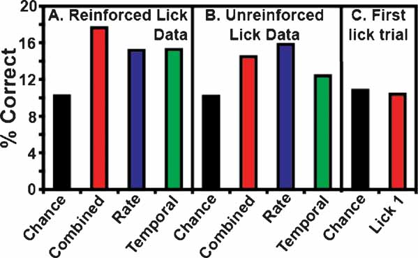
Figure 3. Total ensemble predictions. This figure depicts the total ensemble predictions for all tastants and their concentrations. The percentage of correctly identified taste trials is given on the ordinate. (A) This panel represents tastant predictions for the reinforced lick data. The weighted chance prediction rate is shown in black. The combined model is depicted in red, and the rate and temporal models are given in blue and green, respectively. These conventions are employed for all subsequent figures. Here it is seen that all three model types predict tastants above chance, but the combined model demonstrates the highest prediction level. (B) This panel depicts the tastant predictions as a function of the unreinforced lick data. Again, all three models perform well above chance, but the rate model exhibits the best performance. (C) This panel shows the first unreinforced lick trial (Lick 1) before the start of a tastant block. In this case, the GC neurons cannot anticipate the identity of the upcoming tastant, so the prediction rates for these data are below chance.
Although the GLM predicted the correct outcome 17.6% of the time, this prediction level may seem modest. However, one must consider that there are 17 choices, and in some cases the concentrations are quite close (like the differences between 0.075 and 0.1 M solutions) and in this sense the model performs quite well. Indeed, it is to be expected that as the number of choices decreases, the prediction levels of the model will increase. This will be shown below.
Figure 3 B depicts the percentage of correctly identified tastants given the ensemble activity during the third unreinforced lick. While these ensemble activity patterns did not predict tastants as successfully as the patterns corresponding to the reinforced licks, they nonetheless predicted tastants above chance. Of the three model types for the unreinforced licks, the rate code correctly predicted the most tastants, at an overall level of 15.8%. Under the rate model, 12 of 13 ensembles were capable of discriminating tastants. The combined model ranked second in correctly identifying the stimuli at a rate of 14.5%, and 11 of 13 ensembles could identify tastants with this model. While the total percentage of correctly identified tastants was above chance (10.2%) for the temporal model (12.4%), only 8 of 13 ensembles could predict tastants on this basis. While the activity patterns between the reinforced and unreinforced licks are certainly different (e.g., see Figure 1 ), these results suggest that there is also sufficient information in the unreinforced licks to predict tastants (see below). In this case, it appears that a rate code can adequately convey information about the upcoming tastant delivery, although both a combined code and a temporal code can be used, albeit to a slightly lesser extent, for predicting the delivery of a particular tastant.
As a control for tastant anticipation during the unreinforced licks, the first instance of the third unreinforced lick was also used to predict tastants (denoted as Trial 1 in Figure 3 C). This lick occurs at the start of each block before a given tastant has been delivered, so the subjects should not be able to predict the upcoming stimulus. Indeed, the combined model for this lick predicted tastants at a level of 10.4%, which is actually slightly below the weighted chance value (10.8%). This indicates that the subjects do not anticipate the identity of the upcoming tastant at the start of each block.
Prediction as a Function of Ensemble Size
If ensemble predictions are better than those of single neurons, then it is to be expected that an increase in ensemble size would lead to an increase in prediction levels (Carmena et al., 2003 ; Gutierrez et al., 2006 ; Narayanan et al., 2005 ; Wessberg et al., 2000 ). In Figure 4 we present three representative ensembles, each with 10 neurons, which demonstrate that the prediction probabilities increase as the number of neurons in the ensembles increases. Ensembles 1 and 3 exhibit a slow monotonic increase in probability with increasing size, ensemble 2 shows a large increase in the magnitude of the probability when five or more neurons are used for the predictions.
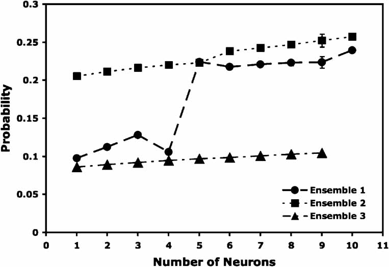
Figure 4. Prediction probability as a function of the number of neurons in an ensemble. Displayed above are the means ± SEMs of the prediction probabilities for three representative ensembles. The number of neurons dropped from each ensemble is displayed on the abscissa, and the corresponding probability is displayed on the ordinate. It should be noted that the SEMs are very small and thus are not visible at most points. The first two ensembles contained 10 neurons, and the third ensemble contained 9 neurons. In the case of ensembles 1 and 3, dropping increasing numbers of neurons causes a monotonic decrease in the prediction probability. Predictions for ensemble 2 remained high until six or more neurons had been removed from the ensemble, after which the probabilities decreased sharply.
We also found that ensembles recorded at the most dorsal level of dysgranular GC usually possessed the greatest prediction strengths. For example, the reinforced lick prediction rates for the first recorded ensembles for each rat were 34.5% (n = 10 neurons), 24.3% (n = 22), 32.4% (n = 10), and 14.1% (n = 27). The corresponding final test sessions for three of these four subjects revealed drops in the prediction rates, with final rates of 9.2% (n = 7), 11.4% (n = 8), 17.5% (n = 15), and 14.3% (n = 23), respectively. In summary, these data indicate that the ensemble predictive value increases with increasing ensemble size but becomes poorer as one descends into the dysgranular cortex, given an initial electrode insertion of 1.3 mm anterior to bregma.
Tastant Predictions During Reinforced Licking
This section is organized into two parts. The first describes the performance of the combined, rate, and temporal models in terms of predicting the individual tastant and concentration combinations. The second explores how well each model classified tastants into categories regardless of concentration.
In these experiments a total of 17 tastants were tested: four concentrations each of MSG, sucrose, and NaCl, two concentrations of citric acid and quinine, and water. A subset of these stimuli was tested during each recording session. The tastant predictions were separated into the percentage of times that each stimulus was correctly identified according to model type (i.e., as combined, rate, or temporal models; see Figure 5 ). As seen in the figure only the combined model (red) correctly identified all 17 stimuli above chance. The rate model (blue) correctly identified thirteen of the 17 stimuli but failed to identify 0.1 M MSG, 0.075 M NaCl, and 0.075 and 0.025 M sucrose above chance levels. The rate model did predict 0.025 M NaCl and 0.0003 M quinine with greater accuracy than the combined model, but in each case this was because a single ensemble dominated the predictions for NaCl (at a level of 50%) or quinine (at a level of 53%). Hence, the prediction levels for these two tastants were inflated. The temporal model (green) correctly predicted fourteen of the stimuli and failed to identify 0.025 M sucrose, 0.005 M citric acid, and 0.0003 M quinine above chance levels.

Figure 5. Tastant predictions for the reinforced lick data. This figure presents the percentage of correctly identified trials for each tastant concentration. The coloring conventions are the same as in Figure 3 . The top graph depicts the predictions for MSG (M) and NaCl (N) at 0.025, 0.075, 0.1, and 0.3 M. The bottom graph depicts the predictions for sucrose (S, at 0.025, 0.075, 0.1, and 0.3 M), citric acid (C, at 0.005 and 0.01 M), and quinine (Q, at 0.0001 and 0.0003 M). Water (W) is repeated in both graphs for comparison with the other stimuli. Of the three model types, only the combined model correctly identified all 17 stimuli above the weighted chance levels.
It is to be expected that the ensemble patterns would be more similar for concentrations of the same tastant than they are to concentrations of a different tastant. Hence, if the models fail to identify the particular concentration of a tastant, then they might predict that a different concentration of the same tastant had been delivered, rather than a different tastant. Moreover, since the number of categories (6) is smaller than the number of tastants (17), we would expect the models’ predictive ability to be improved. To test this hypothesis, we looked at the total number of times that the models correctly predicted the particular tastant category (e.g., NaCl, quinine, etc.), regardless of concentration (see Figures 6 and 7 ). Figure 6 A depicts the overall tastant classifications following the reinforced licks. All three models correctly classified tastant categories above chance, but the combined model exhibited the best performance, with a total prediction level of 34.1%. For the combined model, 11 out of 13 ensembles were capable of classifying tastants above chance levels. The rate model exhibited a slightly lower classification level, and demonstrated an overall prediction level of 32.1%. Ten of thirteen ensembles could correctly identify the tastant category above chance levels. Comparatively, the temporal model demonstrated the weakest performance (31.0%). The overall chance prediction rate was 25.8%. Nine of thirteen ensembles were capable of classifying tastants above chance when a strictly temporal model was used. Figure 7 depicts the classification strength according to tastant category and model type. It can be seen that when either the combined or rate models are used all six tastants are correctly identified above chance. The temporal model correctly identified five of six tastants and failed to identify citric acid.
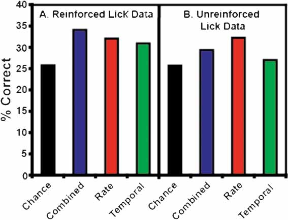
Figure 6. Total tastant classifications. Depicted above are the percentages of correct classifications across all tastant categories. (A) This panel presents the total percentage of correct classifications for the reinforced lick data. All three models classified the tastants into categories regardless of concentration above chance, but the combined model demonstrates the best performance. (B) This panel depicts the total percentage of correct classifications for the unreinforced lick data. Again, all three models classify tastants above chance, but the rate model exhibited the best performance.
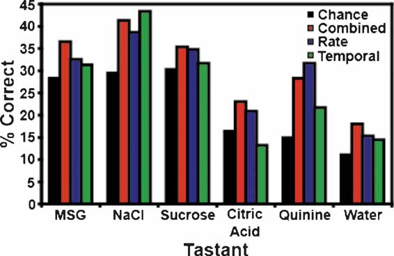
Figure 7. Tastant classifications for the reinforced lick data. This figure breaks down the tastant classification levels according to tastant category. In this case, both the combined and rate models correctly identify all stimuli above the weighted chance levels, while the temporal model fails to identify citric acid.
We note that the predictive aspect of the models improved when the number of variables were reduced from 17 (tastants) to 6 (categories). Continuing in this vein, it is expected that the prediction levels would increase dramatically if only two tastants are compared (Table 1 ). To test this hypothesis, we selected the first ensemble recorded from each animal and then chose the highest concentrations of two tastants for analysis. The first ensembles were selected because they had previously demonstrated the highest prediction rates when all tastants were tested. For the present scenario, the chance rate was 50%. In this case, the same four ensembles described above now achieved prediction rates of 92.9% (for 0.3 M MSG vs. 0.3 M NaCl), 71.4% (0.3 M NaCl vs. sucrose), 66.7%, and 77.3% (both also tested with 0.3 M MSG and 0.3 M NaCl). Therefore, this class of models can identify stimuli at a very high level, although the prediction rates do scale with the number of stimuli (as does chance). We note that trained rats can discriminate between all of these stimuli (Stapleton et al., 2002 ; Stapleton et al., 1999 ).
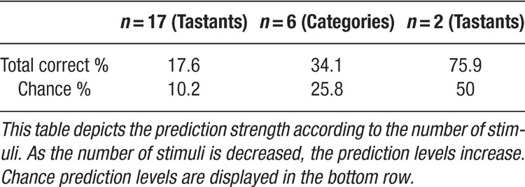
Table 1. Prediction strength as a function of stimulus number, n
Single Neuron Contributions to the Ensembles
From the above it is evident that some ensembles are better predictors of tastants than others. Likewise, in each ensemble different neurons might contribute different amounts of information towards tastant discrimination. To determine how much information single neurons contribute to an ensemble, three ensembles were selected whose prediction rates ranged from about 24–35% (see Figure 8 ). There are many “types” of neurons in the GC including those that were previously identified as chemosensory (Stapleton et al., 2006 ). Figure 8 presents the tastant probabilities associated with the chemosensory neurons in one of these ensembles. Each panel depicts a stripchart of probabilities for a given tastant. The neuron number is given on the ordinate and the probability is given on the abscissa. Each point represents the probability that a tastant occurred given the neural firing pattern on a particular trial, and each row of points represents the probabilities assigned by that neuron to multiple deliveries of that tastant. The dashed vertical lines indicate the chance level of performance for this particular ensemble that contained four chemosensory neurons. Probabilities greater than chance lie to the right of the vertical dashed line, and probabilities less than chance lie to the left. If a neuron cannot reliably signal the presence of a given tastant, then its probabilities should cluster at or below chance. If a neuron can represent a particular tastant, then its probabilities should largely cluster above chance.
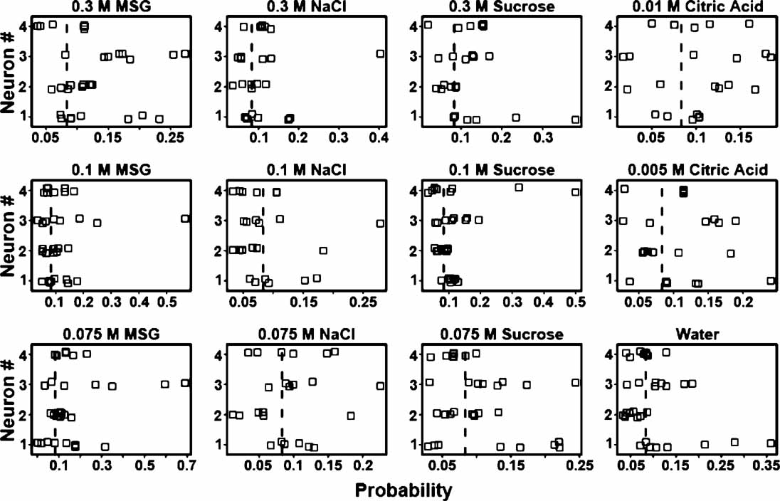
Figure 8. Single trial probabilities for the chemosensory neurons of a representative ensemble. Each panel depicts a stripchart of probabilities for a given tastant, with neuron number (n = 4) given on the ordinate and probability displayed on the abscissa. Each point indicates the probability that a tastant occurred given the firing pattern on a particular trial, and each row of points represents the probabilities assigned by that neuron to multiple deliveries of that tastant. The dashed vertical lines indicate the chance level (8.3%) of performance for this particular ensemble. Probabilities greater than chance lie to the right of the dashed vertical line, and probabilities less than chance lie to the left. On many of the trials these neurons fail to identify the stimuli above chance, but on other trials these neurons respond robustly and to multiple tastants.
The reinforced lick data from each individual neuron were then used to predict the tastants and their particular concentrations. At a particular concentration a tastant is correctly predicted if its associated probability is the greatest in comparison to the other taste stimuli. If across trials a neuron's responses were consistently above chance then those responses reliably contributed to the ensemble's ability to predict the tastant. For example, neuron 3 in Figure 8 would correctly predict 0.075 and 0.3 M MSG and 0.075 M sucrose on most trials, but would not consistently identify 0.1 M NaCl. Note for this neuron, however, that one trial for 0.1 M NaCl would contribute information to the ensemble for the identification of this tastant. In the same manner the responses of this neuron to two trials of 0.075 M sucrose were below chance and hence would not be informative.
Upon investigating the additional ensembles we found that most chemosensory neurons exhibited trial-to-trial variability in the tastant probabilities. We did not see evidence of groups of neurons that were exclusively tuned best to a particular tastant such as sucrose. Instead, the neurons appeared to be responsive to multiple stimuli.
The tastant probabilities for the non-chemosensory neurons of the same ensemble seen in Figure 8 are plotted in Figure 9 . It is evident that many of the probabilities cluster near chance, but it is also clear that these neurons can convey tastant-specific information. An example of this phenomenon is seen in the response of neuron 5 to all three MSG concentrations. These non-chemosensory neurons often correctly identified the tastant on some deliveries but not on others as seen for neuron 6 with 0.3 M sucrose and for neuron 2 with 0.075 M sucrose.
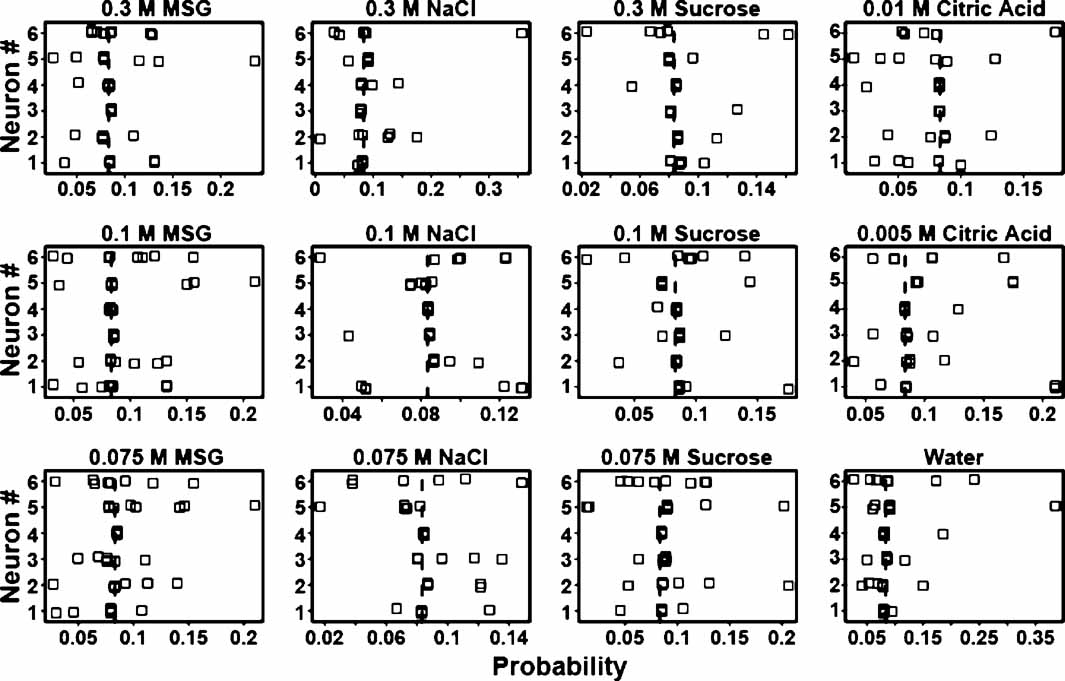
Figure 9. Single trial probabilities for non-chemosensory neurons of the same ensemble. Each panel depicts a stripchart of probabilities for the non-chemosensory neurons (n = 6) of the same ensemble depicted in Figure 8 . Conventions are the same as those in the previous figure. Here most of the tastant probabilities cluster around chance (dashed vertical line), but some neurons do respond above chance to tastants. One example of this is neuron 5, which does respond to many trials of MSG at all concentrations above chance.
Tastant Predictions During Unreinforced Licking
As outlined in the section on the general ensemble predictions, neural activity immediately following the third unreinforced lick can be used to identify tastants above chance. This section further explores these predictions in terms of individual tastant and concentration combinations and also in terms of general tastant classification.
Figure 10 displays the unreinforced lick predictions for each tastant concentration. Conventions are the same as in Figure 5 . None of the three models correctly predicted all stimuli. The combined model correctly identified 12 of 17 tastant concentrations above chance, and failed to predict 0.025 and 0.1 M MSG, 0.3 M NaCl, 0.025 M sucrose, and 0.0003 M quinine. The rate model distinguished 14 of the stimuli but failed to identify 0.025 and 0.1 M MSG and 0.0001 M quinine above chance. The rate model did correctly predict 0.0003 M quinine well above chance, although this is largely due to the influence of a single ensemble (at a level of 57%). Of the three models, the performance of the temporal model was the weakest in that it correctly predicted only 10 of 17 taste stimuli. It failed to identify 0.025, 0.1 and 0.3 M MSG, 0.075 M NaCl, 0.005 and 0.01 M citric acid, and 0.0003 M quinine. On the basis of these data, and those presented in Figure 3 B, it appears that firing rates alone are sufficient to predict most of the future tastant deliveries during the unreinforced licks.
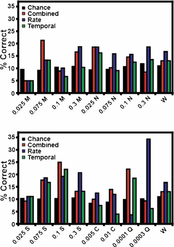
Figure 10. Tastant predictions for the unreinforced lick data. The conventions for this figure are the same as those in Figure 5 . While all three models can correctly identify many of the tastant concentrations above chance, no model correctly identifies all of the stimuli.
Figure 6 B depicts the overall tastant classifications following the unreinforced licks. All three models correctly classified the general tastant type above chance, but the rate model demonstrated the highest prediction level at 32.3%. Note for all models the chance prediction rate was 25.7%. We found that 10 of 13 ensembles could discriminate between tastants on the basis of rate information. Prediction levels for the combined model were about 29.4%, and 11 of 13 models could discriminate between tastants on the basis of the combined information. Hence, the rate and combined models are approximately equivalent in terms of classification ability. Prediction levels for the temporal model were 27.1%, and nine of thirteen ensembles could discriminate between tastant classes on the basis of temporal information alone. The tastant classifications for the unreinforced licks are presented in Figure 11 . Both the combined and rate models correctly identified all stimuli above chance. In contrast, the temporal model only identified three of six stimuli and failed to classify MSG, citric acid, and quinine.
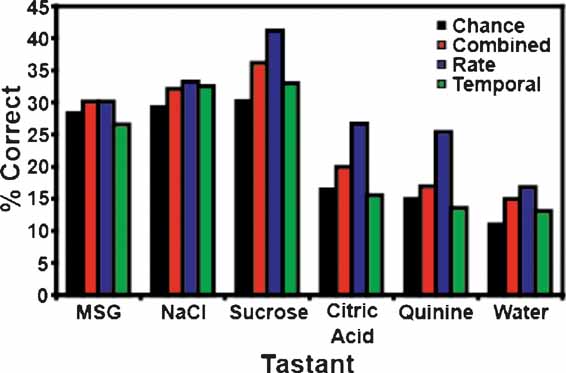
Figure 11. Tastant classifications for the unreinforced lick data. The conventions for this figure are the same as those in Figure 7 . Both the combined and rate models correctly classified all tastant types above the weighted chance levels, but the temporal model failed to identify MSG, citric acid, and quinine.
In the above sections we demonstrated that the first unreinforced lick trial at the start of a new block contained no predictive information about the upcoming tastant (see Figure 3 C). As a second control to determine whether the unreinforced lick data can predict the identity of the upcoming tastant or recall the immediately past tastant, experiments were conducted in which the eight tastant deliveries were randomized within each block (referred to as a random FR5 schedule, see Figure 1 B1B). It can be seen that under these conditions the tastant-evoked responses are rapid and that they return to the baseline rate before the onset of the next unreinforced lick. Hence, the neural activity during the random FR5 schedule is qualitatively similar to that obtained during the normal FR5 test sessions for the reinforced licks.
Similarly, there were no behavioral differences insofar as the lick patterns between the FR5 and random FR5 schedules. As an indicator of lick rate we found that the average time between tastant deliveries within each block was unchanged from the FR5 (3.0 ± 0.6 deliveries/seconds) to the random FR5 (8.1 ± 9.2 deliveries/seconds) (unpaired t test p > 0.15). Hence, lick rate information should not differentially influence the ensemble tastant predictions for the FR5 and random FR5 groups.
Two ensembles were obtained from different rats tested under the random FR5 schedule. The first ensemble contained 11 neurons and the second contained seven neurons. Chance prediction rates for both ensembles were 8.3%. The combined model for the reinforced lick data of first ensemble correctly identified tastants above chance at a level of ∼13%, while the second model correctly identified the stimuli at a level of 5.5%, which is below chance. It should be noted, however, that the rate model of the reinforced lick data for the second model did discriminate tastants at a level of 12.3%. Hence, the reinforced lick data obtained during the random FR5 schedule could be used to predict tastants.
When the unreinforced lick data were used, the total prediction rate across the two ensembles was 5.5%, which is below chance (8.3%). Therefore, when tastant delivery is randomized, the neural activity during the unreinforced licks does not predict the upcoming tastant.
The possibility remained that the unreinforced lick data could predict the previous tastant delivery, in part due to residual tastant activation in the mouth and in part due to its storage in short term memory. Hence, the unreinforced lick data derived from the random FR5 schedule were reanalyzed as a function of the previous tastant delivered. Neither ensemble could predict the previous tastant above chance, with a total prediction level of 7.9%. Because the unreinforced lick data obtained under the random FR5 schedule cannot predict the previous tastant, it is unlikely that the unreinforced lick data from the initial experiments predict tastants on the basis of the previous lick.
Discussion
It is well established that within a single lick (∼150 ms) trained rats can discriminate between tastants (Halpern and Marowitz, 1973 ; Halpern and Tapper, 1971 ). Here we recorded the ensemble firing patterns obtained from GC neurons while trained rats received tastants on FR5 and random FR5 schedules. We modeled the spike trains with a Bayesian GLM and found that small ensembles of GC neurons can predict tastants and their concentrations on the basis of a single lick. Moreover, when the stimulus delivery is predictable, the ensemble firing patterns “anticipate” the upcoming tastant.
Testing on the FR5 Schedule
Given that rats can discriminate between tastants in a single lick, the three models were constructed with 150 ms spike trains. We chose to utilize a fixed ratio test schedule because the activity elicited by licking for tastants could be compared to the activity for licking alone. In addition, the FR5 schedule permitted us determine whether the unreinforced licks could predict the identity of the upcoming tastant. In a more natural environment, rats would lick fluids continuously and not on an FR5 schedule, so the GC should receive a longer stream of information about tastant identity. If our subjects were permitted to lick continuously for tastants, it is likely that the additional neural information would boost our prediction levels. Additionally, our subjects are not required to discriminate between the tastants, so the tastants have no meaning to the subjects other than their hedonic values. If the subjects were forced to attend to the stimuli during a more demanding behavioral task then the corresponding spike trains would be likely to discriminate between the tastants to a greater extent (McAdams and Maunsell, 1999 ; Reynolds et al., 2000 ).
Measuring the Model's Performance
Most studies of ensemble coding typically examine a small number of stimuli and hence have higher prediction rates than those described in the current study (Cohen and Nicolelis, 2004 ; Gutierrez et al., 2006 ; Krupa et al., 2004 ). It should be noted that most of the ensembles were tested with 8–12 tastants. This meant that the model had to discriminate between a large number of stimuli, and chance levels (i.e., 12.5 or 8.3%, etc.) were adjusted according to the number of stimuli tested for each ensemble. In comparison to the overall weighted chance level of 10.2%, the combined prediction rate for the reinforced lick data was 17.6%, or nearly double that of chance. Given that the combined model could also correctly identify all 17 tastant and concentration combinations above chance, this rate of performance is quite good. When the model segregated the tastants into the six categories, the combined prediction rate increased to 34.1% with a weighted chance level of 25.8%. When only two tastants were considered, the performance of the ensembles ranged from 67 to 93%, with a chance level of 50% (Table 1 ). Hence, as the number of stimuli decreased, the prediction rates increased, and the final set of predictions indicate that the model can robustly identify stimuli even with a single lick.
Interestingly, we found that for three of four rats the first set of ensembles predicted tastants more accurately in comparison to ensembles recorded later and therefore at lower depths in the dysgranular cortex. Hence, it is possible that the dorsal pole of GC responds better to taste stimuli relative to the ventral area, suggesting the occurrence of regional differences in taste sensitivity throughout GC (Yamamoto et al., 1984 ). Another possibility is that advancing the electrodes further into GC could produce damage that might disrupt normal functioning.
As seen in Figure 4 we found that the prediction rates increased with increasing ensemble size (Carmena et al., 2003 ; Gutierrez et al., 2006 ; Narayanan et al., 2005 ; Wessberg et al., 2000 ). What is of particular interest is that the ensembles obtained from upper portions of GC predicted tastants more accurately than those more ventrally. Although the reasons for this are unknown, one possibility is that the number of chemosensory neurons is not homogeneously distributed (Yamamoto et al., 1984 ).
Rate and Temporal Information are Important for Tastant Discrimination
Information about tastant identity is conveyed throughout the gustatory neuraxis in terms of both firing rates and temporal response patterns (Di Lorenzo et al., 2003 ; Di Lorenzo and Victor, 2003 ; Jones et al., 2006 ; Simon et al., 2006 ). In these experiments we modeled the firing rates as a function of both rate and temporal parameters. This enabled us to quantify how much information both parameters could convey independently and to determine how the information from these components could be combined to code for tastant identity. When considered alone, the rate and temporal models predicted tastants at an approximately equivalent level. If the temporal and rate parameters carry completely different streams of information, then combining these terms into a single model should cause the prediction level to double. When these parameters were considered simultaneously, however, the combined prediction rate only rose by a couple of percentage points, suggesting significant redundancy in the information carried by the rate and temporal components. Nevertheless, we note that only the combined model could correctly identify all tastants at all concentrations, indicating that both components provide information necessary for tastant discrimination.
Small Ensembles of Neurons Can Classify Tastants
It is expected that the firing patterns for different concentrations of the same tastant should be more similar to each other than they are to other tastants (Ganchrow and Erickson, 1970 ; Stopfer et al., 2003 ). Hence, if the model fails to correctly predict a given taste stimulus, then it might simply predict that a different concentration of the same tastant had been presented rather than guessing that the stimulus was a completely different tastant. We found that for the reinforced lick data the total number of correct predictions was greater than chance for all three models. This suggests that there are some commonalities in the ensemble firing patterns for different concentrations of the same tastant.
Upcoming Tastant Deliveries are Anticipated by GC Neurons
Previous work in the rat GC has revealed the presence of “anticipatory” neurons that increase their firing rates before the subjects begin a licking bout (Stapleton et al., 2006 ; Yamamoto et al., 1988 ). Similarly, neurons in the insular-opercular region of the macaque respond to the approach of a tastant-containing syringe (Plata-Salaman et al., 1992 ; Scott et al., 1991 ; Smith-Swintosky et al., 1991 ).
Several experiments were performed to determine if ensembles of GC neurons could forecast the tastant to be delivered when the stimulus delivery is predictable. For the first set of experiments a single tastant was delivered eight times within a block. Because of this, the subjects maybe be able predict (or time the delivery of) the future tastants within each block (Buhusi and Meck, 2005 ). In this regard, when the ensemble firing patterns corresponding to the unreinforced licks were analyzed, it was found that these patterns could predict the upcoming tastant delivery well above chance (Figure 3 B). Importantly, the unreinforced lick at the start of the tastant block did not contain sufficient information to predict the next tastant (Figure 3 C), presumably because the subject could not know what tastant would be delivered at the beginning of each block. As a second experiment to determine whether predictive information is present in unreinforced licks, the tastant deliveries within each block were randomized so that within each block the subjects should be unable to predict the upcoming tastant. Correspondingly, during the random FR5 experiments the ensemble firing patterns for the unreinforced licks failed to predict the future tastant above chance. The possibility remained, however, that ensembles were responding to residual stimulation of the oral cavity from the previous tastant delivery during the unreinforced licks instead of predicting the future delivery. However, the ensemble firing patterns for the unreinforced licks also failed to predict the previous tastant delivered during the random FR5 schedule. This rules out the possibility that the ensembles respond to residual tastant stimulation during the unreinforced licks. Collectively these data support the conclusion that ensembles of GC neurons can predict the identity of future tastants when such stimuli are delivered in blocks.
We then asked whether the information found in the ensembles could predict the future tastant delivery. One possibility is that the GC sets up a pattern of activity that is an approximation of the future stimulus (Gutierrez et al., 2006 ). Of the three model types, the rate model had the highest prediction level as compared to the combined or temporal models for the unreinforced lick data. The prediction levels between the combined and rate models were not significantly different, while both models are different from the temporal model. Because the combined and temporal models do not differ, changes in firing rate alone are sufficient to signal the identity of the upcoming tastant. In our prior study we found neurons that we classified as “tastant-modulated.” Such neurons did not discriminate between reinforced and unreinforced licks, but these neurons did have different overall firing rates for different tastants (Stapleton et al., 2006 ). We posit that these neurons contributed to the ensemble tastant discriminations during the unreinforced licks on the basis of rate information.
Information Distribution Across the Ensembles
Many studies have found that GC neurons are broadly tuned (Katz et al., 2001 ; Smith-Swintosky et al., 1991 ; Stapleton et al., 2006 ). This property suggests that the gustatory coding mechanism is more consistent with a distributed pattern rather than a labeled line. Indeed, when the GC responses were analyzed with a neural network, it was found that pruning the network did not preferentially degrade the discrimination of a particular tastant, suggesting that the neurons participated in the encoding of more than one taste quality (Nagai et al., 1995 ).
When the single trial probabilities that chemosensory neurons assigned to each tastant delivery were examined (Figure 8 ), it was found that on some trials the neurons correctly predicted a given stimulus well above chance, whereas on other trials the individual predictions were below chance levels. Given the variability in the responses, it is unlikely that these neurons were organized into dedicated channels (labeled lines). Rather, the neurons contributed information about the identity of multiple tastants even though their responses were noisy to various degrees in the single trials. The non-chemosensory neurons within the ensemble also contributed information about the tastants’ identity and concentration (Figure 9 ). Like the chemosensory neurons, these neurons responded well to a given tastant on some trials but not others. It did not appear either that these neurons were organized into particular channels. As noted, many of these neurons were tastant modulated and hence probably assisted in tastant discrimination.
Conclusion
In conclusion, these results indicate that small ensembles of GC neurons can discriminate between tastants on the basis of a single lick, that they utilize both temporal and rate information, and that when tastants are repetitively delivered in blocks ensembles contain information about the identity of the upcoming tastant.
Conflict of Interest Statement
The authors declare that the research was conducted in the absence of any commercial or financial relationships that could be construed as a potential conflict of interest.
Acknowledgements
The authors would like to thank Jim Meloy and Gary Lehew for constructing electrodes and for providing technical support. This work was supported in part by NIH grant DC-01065 and Philip Morris International and Philip Morris USA.
References
Accolla, R., Bathellier, B., Petersen, C. C. H., and Carleton, A. (2007). Differential spatial representation of taste modalities in the rat gustatory cortex. J. Neurosci. 27, 1396-1404.
Balleine, B. W., and Dickinson, A. (2000). The effect of lesions of the insular cortex on instrumental conditioning: evidence for a role in incentive memory. J. Neurosci. 20, 8954-8964.
Baylis, L. L., and Rolls, E. T. (1991). Responses of neurons in the primate taste cortex to glutamate. Physiol. Behav. 49, 973-979.
Bermudez-Rattoni, F., Okuda, S., Roozendaal, B., and McGaugh, J. L. (2005). Insular cortex is involved in consolidation of object recognition memory. Learn. Mem. 12, 447-449.
Buhusi, C. V., and Meck, W. H. (2005). What makes us tick? Functional and neural mechanisms of interval timing. Nat. Rev. Neurosci. 6, 755-765.
Carmena, J. M., Lebedev, M. A., Crist, R. E., Doherty, J. E., Santucci, D. M., Dimitrov, D. F., Patil, P. G., Henriquez, C. S., and Nicolelis, M. A. L. (2003). Learning to control a brain-machine interface for reaching and grasping by primates. PLoS Bio. 1, e42.�
Cerf-Ducastel, B., Van de Moortele, P. F., MacLeod, P., Le Bihan, D., and Faurion, A. (2001). Interaction of gustatory and lingual somatosensory perceptions at the cortical level in the human: a functional magnetic resonance imaging study. Chem. Senses 26, 371-383.
Cohen, D., and Nicolelis, M. A. L. (2004). Reduction of single-neuron firing uncertainty by cortical ensembles during motor skill learning. J. Neurosci. 24, 3574-3582.
De Araujo, I. E., and Rolls, E. T. (2004). Representation in the human brain of food texture and oral fat. J. Neurosci. 24, 3086-3093.
Di Lorenzo, P. M., Hallock, R. M., and Kennedy, D. P. (2003). Temporal coding of sensation: mimicking taste quality with electrical stimulation of the brain. Behav. Neurosci. 117, 1423-1433.
Di Lorenzo, P. M., and Victor, J. D. (2003). Taste response variability and temporal coding in the nucleus of the solitary tract of the rat. J. Neurophysiol. 90, 1418-1431.
Dobson, A. J. (2002). An introduction to generalized linear models, 2nd edn (Boca Raton Chapman & Hall/CRC).
Fontanini, A., and Katz, D. B. (2006). State-dependent modulation of time-varying gustatory responses. J. Neurophysiol. 96, 3183-3193.
Ganchrow, J. R., and Erickson, R. P. (1970). Neural correlates of gustatory intensity and quality. J. Neurophysiol. 33, 768-783.
Gutierrez, R., Carmena, J. M., Nicolelis, M. A. L., and Simon, S. A. (2006). Orbitofrontal ensemble activity monitors licking and distinguishes among natural rewards. J. Neurophysiol 95, 119-133.
Halpern, B. P., and Marowitz, L. A. (1973). Taste responses to lick-duration stimuli. Brain Res. 57, 473-478.
Halpern, B. P., and Tapper, D. N. (1971). Taste stimuli: quality coding time. Science 171, 1256-1258.
Jones, L. M., Fontanini, A., and Katz, D. B. (2006). Gustatory processing: a dynamic systems approach. Curr. Opin. Neurobiol.
Katz, D. B., Simon, S. A., and Nicolelis, M. A. (2001). Dynamic and multimodal responses of gustatory cortical neurons in awake rats. J. Neurosci. 21, 4478-4489.
Katz, D. B., Simon, S. A., and Nicolelis, M. A. (2002). Taste-specific neuronal ensembles in the gustatory cortex of awake rats. J. Neurosci. 22, 1850-1857.
Kosar, E., Grill, H. J., and Norgren, R. (1986). Gustatory cortex in the rat. I. Physiological properties and cytoarchitecture. Brain Res. 379, 329-341.
Krupa, D. J., Wiest, M. C., Shuler, M. G., Laubach, M., and Nicolelis, M. A. L. (2004). Layer-specific somatosensory cortical activation during active tactile discrimination. Science 304, 1989-1992.
McAdams, C. J., and Maunsell, J. H. (1999). Effects of attention on orientation-tuning functions of single neurons in macaque cortical area V4. J. Neurosci. 19, 431-441.
Miyaoka, Y., and Pritchard, T. C. (1996). Responses of primate cortical neurons to unitary and binary taste stimuli. J. Neurophysiol. 75, 396-411.
Nagai, T., Katayama, H., Aihara, K., and Yamamoto, T. (1995). Pruning of rat cortical taste neurons by an artificial neural network model. J. Neurophysiol. 74, 1010-1019.
Narayanan, N. S., Kimchi, E. Y., and Laubach, M. (2005). Redundancy and synergy of neuronal ensembles in motor cortex. J. Neurosci. 25, 4207-4216.
Nicolelis, M. A., Dimitrov, D., Carmena, J. M., Crist, R., Lehew, G., Kralik, J. D., and Wise, S. P. (2003). Chronic, multisite, multielectrode recordings in macaque monkeys. Proc. Natl. Acad. Sci. USA 100, 11041-11046.
Nitschke, J. B., Dixon, G. E., Sarinopoulos, I., Short, S. J., Cohen, J. D., Smith, E. E., Kosslyn, S. M., Rose, R. M., and Davidson, R. J. (2006). Altering expectancy dampens neural response to aversive taste in primary taste cortex. Nat. Neurosci. 9, 435-442.
Ogawa, H., and Wang, X. D. (2002). Neurons in the cortical taste area receive nociceptive inputs from the whole body as well as the oral cavity in the rat. Neurosci. Lett. 322, 87-90.
Plata-Salaman, C. R., Scott, T. R., and Smith-Swintosky, V. L. (1992). Gustatory neural coding in the monkey cortex: L-amino acids. J. Neurophysiol. 67, 1552-1561.
Reynolds, J. H., Pasternak, T., and Desimone, R. (2000). Attention increases sensitivity of V4 neurons. Neuron. 26, 703-714.
Scott, T. R., Plata-Salaman, C. R., Smith, V. L., and Giza, B. K. (1991). Gustatory neural coding in the monkey cortex: stimulus intensity. J. Neurophysiol. 65, 76-86.
Sewards, T. V. (2004). Dual separate pathways for sensory and hedonic aspects of taste. Brain Res. Bull. 62, 271-283.
Simon, S. A., de Araujo, I. E., Gutierrez, R., and Nicolelis, M. A. (2006). The neural mechanisms of gustation: a distributed processing code. Nat. Rev. Neurosci. 7, 890-901.
Small, D. M., Gregory, M. D., Mak, Y. E., Gitelman, D., Mesulam, M. M., and Parrish, T. (2003). Dissociation of neural representation of intensity and affective valuation in human gustation. Neuron. 39, 701-711.
Smith-Swintosky, V. L., Plata-Salaman, C. R., and Scott, T. R. (1991). Gustatory neural coding in the monkey cortex: stimulus quality. J. Neurophysiol. 66, 1156-1165.
Soares, E. S., Stapleton, J. R., Rodriguez, A., Fitzsimmons, N., Oliveira, L., Nicolelis, M. A. L., and Simon, S. A. (2007). Behavioral and neural responses to gustatory stimuli delivered non-contingently through intra-oral cannulas. Physiol. & Behav.
Stapleton, J. R., Lavine, M. L., Wolpert, R. L., Nicolelis, M. A. L., and Simon, S. A. (2006). Rapid Taste Responses in the Gustatory Cortex during Licking. J. Neurosci. 26, 4126-4138.
Stapleton, J. R., Luellig, M., Roper, S. D., and Delay, E. R. (2002). Discrimination between the tastes of sucrose and monosodium glutamate in rats. Chem. Senses 27, 375-382.
Stapleton, J. R., Roper, S. D., and Delay, E. R. (1999). The taste of monosodium glutamate (MSG), L-aspartic acid, and N-methyl-D-aspartate (NMDA) in rats: are NMDA receptors involved in MSG taste? Chem. Senses 24, 449-457.
Stopfer, M., Jayaraman, V., and Laurent, G. (2003). Intensity versus identity coding in an olfactory system. Neuron 39, 991-1004.
Verhagen, J. V., Kadohisa, M., and Rolls, E. T. (2004). Primate insular/opercular taste cortex: neuronal representations of the viscosity, fat texture, grittiness, temperature, and taste of foods. J. Neurophysiol. 92, 1685-1699.
Wessberg, J., Stambaugh, C. R., Kralik, J. D., Beck, P. D., Laubach, M., Chapin, J. K., Kim, J., Biggs, S. J., Srinivasan, M. A., and Nicolelis, M. A. L. (2000). Real-time prediction of hand trajectory by ensembles of cortical neurons in primates. Nature 408, 361 365.
Wiesenfeld, Z., Halpern, B. P., and Tapper, D. N. (1977). Licking behavior: evidence of hypoglossal oscillator. Science 196, 1122-1124.
Yamamoto, T., Matsuo, R., and Kawamura, Y. (1980). Localization of cortical gustatory area in rats and its role in taste discrimination. J. Neurophysiol. 44, 440-455.
Yamamoto, T., Matsuo, R., Kiyomitsu, Y., and Kitamura, R. (1988). Sensory inputs from the oral region to the cerebral cortex in behaving rats: an analysis of unit responses in cortical somatosensory and taste areas during ingestive behavior. J. Neurophysiol. 60, 1303-1321.
Yamamoto, T., Matsuo, R., Kiyomitsu, Y., and Kitamura, R. (1989). Taste responses of cortical neurons in freely ingesting rats. J. Neurophysiol. 61, 1244-1258.
Yamamoto, T., Yuyama, N., Kato, T., and Kawamura, Y. (1984). Gustatory responses of cortical neurons in rats. I. Response characteristics. J. Neurophysiol. 51, 616-635.
Keywords: Bayesian generalized linear model, gustatory cortex, neural ensembles, fixed ratio schedule, multi-electrode neurophysiology, rate and temporal coding, gustation, licking
Citation: Jennifer R. Stapleton, Michael. L. Lavine, Miguel A. L. Nicolelis and Sidney A. Simon (2007). Ensembles of gustatory cortical neurons anticipate and discriminate between tastants in a single lick. Front. Neurosci. 1:1. 161-174. doi: 10.3389/neuro.01/1.1.012.2007
Received: 15 August 2007; Paper pending published: 01 September 2007;
Accepted: 01 September 2007;
Published online: 15 October 2007.
Edited by:
Idan Segev, Hebrew University, IsraelReviewed by:
Federico Bermudez-Rattoni, Universidad Nacional Autónoma de México, MexicoMarshall Devor, Hebrew University of Jerusalem, Israel
Copyright: © 2007 Stapleton, Lavine, Nicolelis and Simon. This is an open-access article subject to an exclusive license agreement between the authors and the Frontiers Research Foundation, which permits unrestricted use, distribution, and reproduction in any medium, provided the original authors and source are credited.
*Correspondence: Jennifer Stapleton, Department of Neurobiology, Duke University, Durham, NC 27710, USA. Tel.: +1 (919) 668–6107.