1
Max Planck Institute for Dynamics and Self - Organization, Göttingen, Germany
2
Bernstein Center for Computational Neuroscience Göttingen, Göttingen, Germany
3
Göttingen Graduate School for Neurosciences and Molecular Biosciences, Göttingen, Germany
4
Institute of Higher Nervous Activity and Neurophysiology, Russian Academy of Sciences, Moscow, Russia
5
Department of Neurophysiology, Ruhr - University Bochum, Bochum, Germany
6
Department of Psychology, University of Connecticut, Storrs, CT, USA
Concerted neural activity can reflect specific features of sensory stimuli or behavioral tasks. Correlation coefficients and count correlations are frequently used to measure correlations between neurons, design synthetic spike trains and build population models. But are correlation coefficients always a reliable measure of input correlations? Here, we consider a stochastic model for the generation of correlated spike sequences which replicate neuronal pairwise correlations in many important aspects. We investigate under which conditions the correlation coefficients reflect the degree of input synchrony and when they can be used to build population models. We find that correlation coefficients can be a poor indicator of input synchrony for some cases of input correlations. In particular, count correlations computed for large time bins can vanish despite the presence of input correlations. These findings suggest that network models or potential coding schemes of neural population activity need to incorporate temporal properties of correlated inputs and take into consideration the regimes of firing rates and correlation strengths to ensure that their building blocks are an unambiguous measures of synchrony.
Coordinated activity of neural ensembles contributes a multitude of cognitive functions, e.g., attention (Steinmetz et al., 2000
), encoding of sensory information (Stopfer et al., 1997
; Galan et al., 2006
), stimulus anticipation and discrimination (Zohary et al., 1994
; Vaadia et al., 1995
). Novel experimental techniques allow simultaneous recording of activity from a large number of neurons (Greenberg et al., 2008
) and offer new possibilities to relate the activity of neuronal populations to sensory processing and behavior. Yet, understanding the function of neural assembles requires reliable tools for quantification, analysis and interpretation of multiple simultaneously recorded spike trains in terms of underlying connectivity and interactions between neurons.
As a first step beyond the analysis of single neurons in isolation, much attention has focused on the pairwise spike correlations (Schneidman et al., 2006
; Macke et al., 2009
; Roudi et al., 2009
), their temporal structure and the influence of topology (Kass and Ventura, 2006
; Kriener et al., 2009
; Ostojic et al., 2009
; Tchumatchenko et al., 2010
). Pairwise neuronal correlations are traditionally quantified using count correlations, e.g., correlation coefficients (Perkel et al., 1967
). However, it remains largely elusive how correlations present in the input to pairs of neurons are reflected in the count correlations of their spike trains. What are the signatures of input correlations in the count correlations? And vice versa, what conclusions about input correlations and interactions can be drawn on the basis of count correlations and their changes?
Here we address these questions using a framework of Gaussian random functions. We find that correlation coefficients can be a poor indicator of input synchrony for some cases of input correlations. In particular, count correlations computed for time bins larger than the intrinsic temporal scale of correlations can vanish for some functional forms of input correlations. These potential ambiguities were not reported in previous studies of leaky integrate and fire models which focused on the analytically accessible choice of white noise input currents (de la Rocha et al., 2007
; Shea-Brown et al., 2008
).
The paper is organized as follows: we first introduce several common spike count measures (Section “Materials and Methods”) and the statistical framework (Section “Results”). Then we study the zero time lag correlations (Section “Spike Correlations with Zero Time Lag”) and the influence of the temporal structure of input correlations on measures of spike correlations (Section “Temporal Scale of Spike Correlations”). We show that spike count correlations can vanish despite the presence of input cross correlations (Section “Vanishing Count Covariance in the Presence of Cross Correlations”). Finally, we discuss potential consequences of our findings for the design of population models and the experimentally measured spike correlations.
Measures of Correlation
The spike train si(t) of a neuron i is completely described by the sequence of spike times ti. This description is often simplified using discrete bins of size T (Figure 1
). To describe pairwise spike correlations, several competing measures are used (Perkel et al., 1967
; Svirskis and Hounsgaard, 2003
; Schneidman et al., 2006
; de la Rocha et al., 2007
; Shea-Brown et al., 2008
; Roudi et al., 2009
). Here, we focus on the most commonly used measures of spike correlations: conditional firing rate, correlation coefficient, normalized correlation coefficient and count covariance. We will consider the relation between these measures and their dependence on (1) the underlying input correlation strength, (2) firing rate, (3) temporal structure of spike trains, and (4) size of the time bin used to compute count correlations.
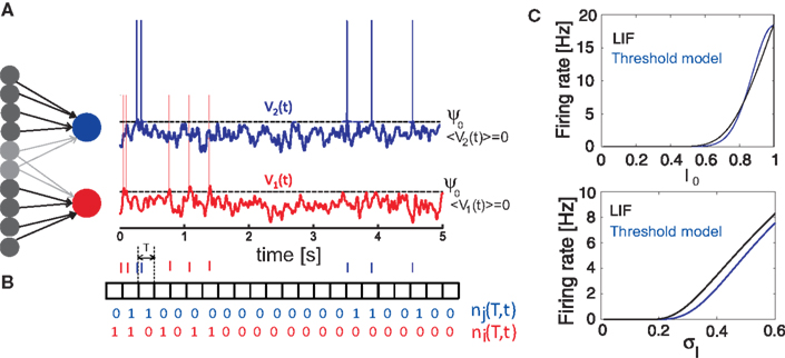
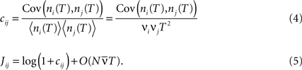
Figure 1. Generation of spike trains and transformation to spike counts. (A) Generation of spike trains from correlated voltage traces of two neurons with common presynaptic partners. (B) Red and blue vertical bars indicate the spike trains of two neurons. Squares show the boundaries of bins with duration T. ni(T,t) and nj(T,t) illustrate corresponding binned spike trains. (C) Firing rate vs. input current in the LIF model (first order solution) and the threshold model (Eq. 11) computed for σI = 0.25 (top), I0 = 0.6 (bottom) and ψ0 = 1, Vr = 0, τM = 15 ms and τI = 5 ms.
The spike timing correlations of two spike trains si(t) and sj(t) are often quantified using the conditional firing rate function νcond,ij(τ) (Binder and Powers, 2001
; Tchumatchenko et al., 2010
):
Here νi and νj are the mean firing rates of neurons i and j, respectively. Correlations within a spike train are described by the auto conditional firing rate νcond(τ).
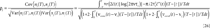
An alternative measure based on count correlations is the correlation coefficient ρij (Perkel et al., 1967
; de la Rocha et al., 2007
; Greenberg et al., 2008
; Shea-Brown et al., 2008
; Tetzlaff et al., 2008
):
where ni(T) and nj(T) are spike counts of neuron i and j measured in synchronous time bins of width T, see Figure 1
. A related measure of pairwise correlations is the normalized correlation coefficient cij (Roudi et al., 2009
). It determines pairwise interactions Jij in maximum entropy models of networks of N neurons with average firing rate  (Schneidman et al., 2006
; Roudi et al., 2009
):
(Schneidman et al., 2006
; Roudi et al., 2009
):
(Schneidman et al., 2006
; Roudi et al., 2009
):
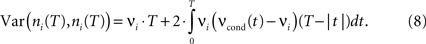
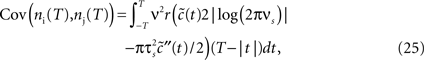
Covariance can be obtained via the integration of cross conditional firing rate νcond,ij (τ) over the time bin T:
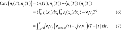
The count variance can be obtained from the auto conditional firing rate νcond(τ):
For bin sizes smaller than the intrinsic time constant (T < τs, see Eq. 14), we can directly relate conditional firing rate νcond,ij(τ) and the correlation coefficient ρij
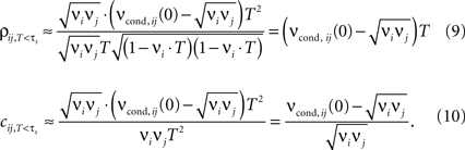
In this limit, the properties of ρij, cij are largely determined by νcond,ij(0). Several experimental studies used bin sizes ranging from T = 0.1 to 1 ms, which are compatible with this T-regime of correlation coefficients (e.g., Lampl et al., 1999
; Takahashi and Sakurai, 2006
).
The quantities presented here all measure different aspects of spike correlations and can potentially have different computational properties. Furthermore, each of the quantities can exhibit a nonlinear dependence on firing rate, input statistics or bin size. Below, we consider these measures of spike correlations, as well as their dependence on firing rate, input statistics and bin size.
To access spike correlations in a pair of neurons, we use the framework of correlated, stationary Gaussian processes to model the voltage potential V(t) of each neuron. This approach generates voltage traces with statistical properties consistent with cortical neurons (Azouz and Gray, 1999
; Destexhe et al., 2003
). The simplest conceivable model of spike generation from a fluctuating voltage V(t) identifies the spike times tj with upward crossings of a threshold voltage (Rice, 1954
; Jung, 1995
; Burak et al., 2009
). The times tj determine the spike train:

where ψ0 is the threshold voltage, and δ(·) and θ(·) are the Dirac delta and Heaviside theta functions, respectively. Each neuron has a stationary firing rate ν = 〈s(t)〉. We model V(t) by a random realization of a stationary continuous correlated Gaussian process V(t) (Azouz and Gray, 1999
; Destexhe et al., 2003
) with zero mean and a temporal correlation function C(τ), which decays for larger time lags τ.

〈·〉 denotes the ensemble average. We assume a smooth C(τ) such that Cn(0) exist for n ≤ 6 and the rate of threshold crossings is finite (Stratonovich, 1964
). All other properties of C(τ) can be freely chosen. This makes our formal description applicable to a large class of models, each of which is characterized by a particular choice C(τ). For simulations using digitally synthesized Gaussian processes (Prichard and Theiler, 1994
) and numerical integration of Gaussian integrals (e.g., Wolfram Research, 2009
) we used a correlation function compatible with power spectra of cortical neurons (Destexhe et al., 2003
):

In cortical neurons in vivo the temporal width of C(τ) can from 10 to 100 ms (Azouz and Gray, 1999
; Lampl et al., 1999
). We characterize the temporal width of C(τ) using the correlation time constant τs:

Note, that the correlation time τs as defined in Eq. 14 is close to a commonly used definition of autocorrelation time 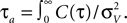 For C(τ) as in Eq. 13 τa = πτs/2. The correlation time τs and the threshold ψ0 determine the firing rate ν:
For C(τ) as in Eq. 13 τa = πτs/2. The correlation time τs and the threshold ψ0 determine the firing rate ν: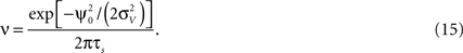
The firing rate ν is the rate of positive threshold crossings, which is equivalent to half of the Rice rate of a Gaussian process (Rice, 1954
). For non-Gaussian processes the rate of threshold crossings can deviate from Eq. 15 and there is no general approach for obtaining ν in this case (Leadbetter et al., 1983
). We note, that the firing rate ν of a neuron depends only on two parameters: the correlation time and the threshold-to-variance ratio, but not on the specific functional choice of the correlation function. Hence, processes with the same correlation time but with a different functional form of C(τ) will have the same mean rate of spikes, though their spike auto and cross correlations can differ significantly. Our framework can be expected to capture neural activity in the regime where the mean time between the subsequent spikes is much longer than the decay time of the spike triggered currents. This occurs if the spikes are sufficiently far apart and the spike decision is primarily determined by the stationary voltage statistics rather than spike evoked currents. Therefore, this model should only be used in the fluctuation driven, low firing rate ν < 1/(2πτs) regime, which is important for cortical neurons (Greenberg et al., 2008
).
The leaky integrate and fire (LIF) model (Brunel and Sergi, 1998
; Fourcaud and Brunel, 2002
) has a similar spike generation mechanism. To compare both models, we study the transformation of input current to spikes. The LIF neuron driven by Ornstein–Uhlenbeck current I(t) with time constant τI can be described by

where τM is the membrane time constant and I0 is the mean input current. When V(t) reaches the threshold ψ0, the neuron emits a spike, and V(t) is reset to Vr. The LIF model mainly differs from our framework by the presence of reset after each spike. For low firing rates, where the reset has little influence on the following spike, the threshold model and the LIF model can be expected to yield equivalent results. In Figure 1
C we compare the first order firing rate approximation (first order in  ) of a LIF neuron driven by colored noise, which can be obtained via involved Fokker–Planck calculations (Brunel and Sergi, 1998
; Fourcaud and Brunel, 2002
) and the firing rate of the corresponding threshold neuron
) of a LIF neuron driven by colored noise, which can be obtained via involved Fokker–Planck calculations (Brunel and Sergi, 1998
; Fourcaud and Brunel, 2002
) and the firing rate of the corresponding threshold neuron  . In general, the details of the spike generating model can have a strong effect on current susceptibility and spike correlations (Vilela and Lindner, 2009
). However, we find that both models have a very similar current susceptibility for a range of input currents and spike correlations derived in the forthcoming sections are consistent with the corresponding correlations in the LIF model, e.g., firing rate dependence of weak cross correlations (de la Rocha et al., 2007
; Shea-Brown et al., 2008
), the influence of noise mean and variance on the firing rates and spike correlations (Brunel and Sergi, 1998
; de la Rocha et al., 2007
; Ostojic et al., 2009
), sublinear dependence of correlation coefficients on input strength (Moreno-Bote and Parga, 2006
; de la Rocha et al., 2007
).
. In general, the details of the spike generating model can have a strong effect on current susceptibility and spike correlations (Vilela and Lindner, 2009
). However, we find that both models have a very similar current susceptibility for a range of input currents and spike correlations derived in the forthcoming sections are consistent with the corresponding correlations in the LIF model, e.g., firing rate dependence of weak cross correlations (de la Rocha et al., 2007
; Shea-Brown et al., 2008
), the influence of noise mean and variance on the firing rates and spike correlations (Brunel and Sergi, 1998
; de la Rocha et al., 2007
; Ostojic et al., 2009
), sublinear dependence of correlation coefficients on input strength (Moreno-Bote and Parga, 2006
; de la Rocha et al., 2007
).
) of a LIF neuron driven by colored noise, which can be obtained via involved Fokker–Planck calculations (Brunel and Sergi, 1998
; Fourcaud and Brunel, 2002
) and the firing rate of the corresponding threshold neuron . In general, the details of the spike generating model can have a strong effect on current susceptibility and spike correlations (Vilela and Lindner, 2009
). However, we find that both models have a very similar current susceptibility for a range of input currents and spike correlations derived in the forthcoming sections are consistent with the corresponding correlations in the LIF model, e.g., firing rate dependence of weak cross correlations (de la Rocha et al., 2007
; Shea-Brown et al., 2008
), the influence of noise mean and variance on the firing rates and spike correlations (Brunel and Sergi, 1998
; de la Rocha et al., 2007
; Ostojic et al., 2009
), sublinear dependence of correlation coefficients on input strength (Moreno-Bote and Parga, 2006
; de la Rocha et al., 2007
).We include cross correlation between two spike trains i and j via a common component in Vi(t) and Vj(t), r > 0:
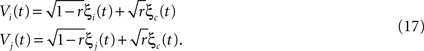
where ξc denotes the common component and ξi, ξj are the individual noise components. In a Gaussian ensemble any expectation value is determined by pairwise covariances only. Thus all pairwise correlations are determined by the joint Gaussian probability density  of
of 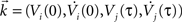 , where
of , where
Matrix entries are covariances Cxy = 〈kxky〉 with Cij = rC(τ). Below, we calculate the conditional firing rate νcond,ij(τ) (Eqs 1 and 11) for several important limits.
Spike Correlations with Zero Time LAG
The above framework allows one to derive an analytical expression for the cross conditional firing rate with zero time lag, νcond,ij(0). Via Eqs 5, 9 and 10 νcond,ij(0) can be related to cij, ρij and Jij. For a pair of statistically identical neurons with (ν = ν1 = ν2). νcond,ij(0) in Eq. 1 can be solved by transforming the correlation matrix C (Eq. 18) into a block diagonal form via a variable transformation:
The matrix C is then the identity matrix for τ = 0, and  We obtain:
We obtain: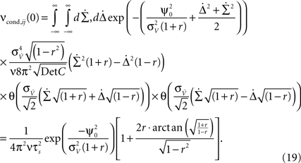
Equation 19 (Figure 3
A) shows, as expected, that νcond,ij(0) increases with increasing strength of input correlations r. Since both correlation coefficients ρij, and normalized correlation coefficient cij are proportional to νcond,ij(0) (Eqs 9 and 10), both measures also increase with increasing r, which is consistent with experimental findings (Binder and Powers, 2001
; de la Rocha et al., 2007
). However, the functional form of r-dependence and the sensitivity to the firing rate ν of cij and ρij are different (Figure 2
). The normalized correlation coefficient cij and pairwise coupling Jij are both inversely proportional to ν, and thus decrease with increasing ν for any value of r (Eqs 4 and 5; Figure 2
B). Notably, we find that cij can be normalized to cij → cij· (νT) to yield a less ambiguous measure of the input correlation strength (Eqs 4 and 10; Figures 3
C,D). Additionally, we find that the firing rate dependence of ρij is different for the weak and strong correlations.
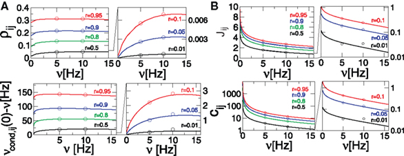
Figure 2. Dependence of correlation coefficient ρij and conditional rate νcond,ij(0) on firing rate and correlation strength. (A, top) ρij vs. ν, (A, bottom) νcond,ij(0) vs. ν, as in Eq. 19. (B, top) Pairwise couplings Jij vs. ν, as in Eq. 5. (B, bottom) cij vs. ν. All quantities are computed for τs = 10 ms, C(τ) as in Eq. 13 and ν = ν1 = ν2; circles denote the corresponding simulation results. ρij, cij and Jij are computed for T = τs/4.
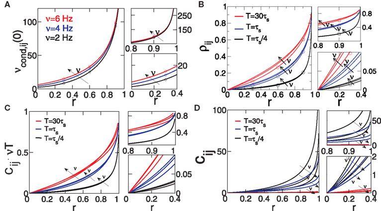
Figure 3. Dependence of spike correlation measures on firing rate ν and correlation strength r. (A) νcond,ij(0) vs. r (B) ρij vs. r for bin widths T = 30τs (red), T = τs (blue), T = τs/4 (black). (C) cij νT vs. r. (D) cij vs. r. All quantities are computed for C(τ) as in Eq. 13, correlation time τs = 10 ms and three firing rates ν = 2, 4, 6 Hz, ν = ν1 = ν2; circles denote simulation results for the corresponding parameters.
Equation 19 further exposes one important feature of νcond,ij(0), and thus of cij and ρij for small time bins: all three measures depend on the temporal scale of the input correlations (τs), but not on the functional form of input correlation C(τ). Thus, changes in νcond,ij(0) and correlation coefficient ρij can be interpreted as a change of the strength of underlying input correlation strength, if a firing rate modification can be excluded.
In the linear r-regime, the analytical expression for νcond,ij(0) can be further simplified:

In this limit, νcond,ij(0) shows a strong dependence on the firing rate ν (Figure 3
A, right, Figure 2
A, top). This dependence is remarkably similar to the firing rate dependence found previously in vitro and in vivo in cortical neurons and LIF models (de la Rocha et al., 2007
; Greenberg et al., 2008
; Shea-Brown et al., 2008
).
In the limit of strong input correlations, Eq. 19 can be simplified to:

In this regime, νcond,ij(0) does not depend on the firing rate ν (Amari, 2009
). Furthermore, for strong input correlations and small bin sizes T the correlation coefficient ρij also changes only marginally over a range of firing rates (0 < ν < 15 Hz, Figure 2
A), since it depends linearly on νcond,ij(0). Note, as r is approaching 1 the temporal width of νcond,ij(τ) is approaching 0 and the peak νcond,ij(0) diverges, corresponding to the delta peak in the autoconditional firing rate νcond(τ) which results from the self-reference of a spike. For r ≈ 1, almost every spike in one train has a corresponding spike in the other spike train, however these two are jittered. The temporal jitter of the spikes can be characterized by the peak of the conditional firing rate  and its temporal width
  both of which are threshold and firing rate independent in this limit. Notably, the threshold independence and the dependence on temporal scale of input correlations are consistent with previous experimental findings on spike reliability (Mainen and Sejnowski, 1995
).
both of which are threshold and firing rate independent in this limit. Notably, the threshold independence and the dependence on temporal scale of input correlations are consistent with previous experimental findings on spike reliability (Mainen and Sejnowski, 1995
).
and its temporal width both of which are threshold and firing rate independent in this limit. Notably, the threshold independence and the dependence on temporal scale of input correlations are consistent with previous experimental findings on spike reliability (Mainen and Sejnowski, 1995
).Temporal Scale of Spike Correlations
So far we considered only spike correlations occurring with zero time lag. However, spike correlations can also span across significant time intervals (Azouz and Gray, 1999
; Destexhe et al., 2003
). The temporal structure of spike correlations, as reflected in the conditional firing rate νcond,ij(τ), can induce temporal correlations within and across time bins and could potentially alter count correlations. To capture correlations with a non-zero time lag, spike correlation measures are calculated for time bins T spanning tens to hundreds of milliseconds, e.g., 20 ms (Schneidman et al., 2006
), 30–70 ms (Vaadia et al., 1995
), 192 ms (Greenberg et al., 2008
) and 2 s (Zohary et al., 1994
). For time bins longer than the time constant of the input correlations, measures of correlations become sensitive to the temporal structure of νcond,ij(τ). Moreover, the values of ρij and cij depend on the bin size T used for their calculation. Figure 3
shows how dependence of ρij and cij on the firing rate is altered by a change in bin size. Increasing the bin size leads to the increase of the calculated correlation coefficient ρij, and also increases the sensitivity of ρij to the firing rate. The fact that increasing T brings the calculated correlation coefficient closer to the underlying input correlation r could justify the use of long time bins in the above studies. But do correlation coefficients always increase with increasing time bins? To further clarify how the temporal structure of input correlations influences the temporal correlations within and across spike trains, we investigate the covariance of spike counts recorded at different times
where ni(T, t) and ni(T, t + τ) are the spike counts of neurons i, j measured in time bins of the same duration T, but shifted by the time lag τ. For each time lag τ, covariance of the spike counts can be calculated using νcond,ij(τ) (Eq. 1). Below, we will first address the temporal structure of auto correlations in a spike train, and then consider the cross correlations between spike trains.
The auto conditional firing rate νcond(τ)
For large time lags τ we expect the auto conditional firing rate to approach the stationary rate but to deviate from it significantly for small time lags. Of particular importance for population models is the limit of small but finite τ, which determines the time scale on which adjacent time bins are correlated. At τ = 0, the auto conditional firing rate has a δ-peak reflecting the trivial auto correlation of each spike with itself. In the limit of small but finite time lag (0 < τ < τs) we find a period of intrinsic silence, where the leading order ∝τ4 is independent of a particular functional choice of C(τ). We solve νcond(τ) (Eq. 2) by transforming the correlation matrix in Eq. 18 into a block diagonal form using new variables
Then only few elements of the corresponding symmetric density matrix  remain non-zero: the diagonal elements
  i ∈ {1, 2, 3, 4} and the non-diagonal elements
remain non-zero: the diagonal elements i ∈ {1, 2, 3, 4} and the non-diagonal elements
For C(τ) as in Eq. 13 we obtain a simple analytical expression in the limit of 0 < τ < τs:
This equation shows that νcond(τ) depends on the temporal structure of a neuron’s input and firing rate, Figure 4
B. Respectively, the silence period after each spike depends on the functional form and time constant of the voltage correlation function C(τ) and firing rate (Figures 4
B and 5
A). Figure 4
B illustrates νcond(τ) obtained using numerical integration of Gaussian probability densities (e.g., Wolfram Research, 2009
), νcond(τ) obtained from simulations of digitally synthesized Gaussian processes (Prichard and Theiler, 1994
) and the τ < τs approximation in Eq. 23. In this framework, the silence period after each spike mimics the refractoriness present in real neurons (Dayan and Abbott, 2001
).
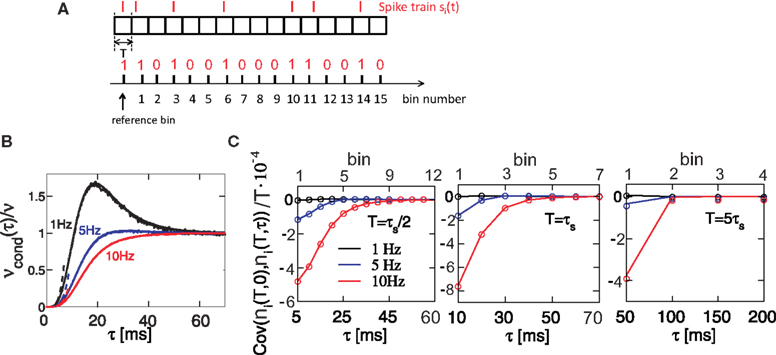
Figure 4. Spike correlations and count correlations within a spike train. (A) Example of a binned spike train si(t), bins numbered with respect to a reference time bin. (B) νcond(τ) vs. τ for τ = 10 ms, numerical solution and simulations for the firing rates ν = 1 Hz (black), 5 Hz (blue) and ν = 10 Hz (red) are superimposed. Dotted lines denote the corresponding solutions for small τ (Eq. 23). (C) Cov(ni(T,0),nj(T,τ))/T vs. τ for τs = 10 ms, time bin T = τs/2 = 5 ms (left), T = 10 ms = τs (middle), T = 5τs = 50 ms (right). Circles denote the corresponding simulation points, adjacent time bins are denoted by the first points on the time axis. All spike correlations are computed for C(τ) as in Eq. 13.
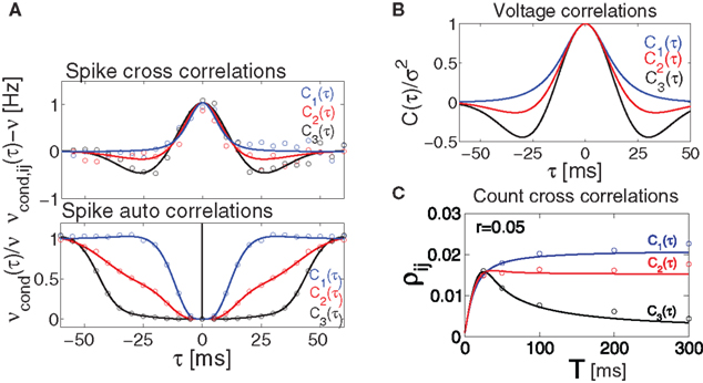
Figure 5. Influence of temporal structure on pairwise spike correlations. (A) Spike cross correlations νcond,ij(τ) and auto correlations νcond(τ) for three voltage correlation functions Ci(τ). (B) Voltage correlations 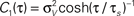 (blue),
  (red),
  (black). Note, all voltage correlations Ci(τ) share the same correlation time τs but have a different functional form. (C) ρij vs. T for voltage correlation functions Ci(τ). For all figures the correlation time τs = 10 ms, ν = 5 Hz, ν = ν1 = ν2; circles denote the corresponding simulation points.
(blue), (red), (black). Note, all voltage correlations Ci(τ) share the same correlation time τs but have a different functional form. (C) ρij vs. T for voltage correlation functions Ci(τ). For all figures the correlation time τs = 10 ms, ν = 5 Hz, ν = ν1 = ν2; circles denote the corresponding simulation points.Count correlations within a spike train
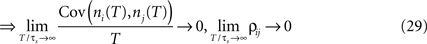
Here we study how the input correlations shape the temporal structure of spike autocorrelations. In particular, we focus on how the input correlations and spike autocorrelations are reflected in count correlations within a spike train. The silence period after a spike is reflected in vanishing νcond(τ) for 0 < τ < τs and results in negative covariation of spike counts in adjacent time bins. We find that the relation between νcond(τ) and spike count covariance is most salient for higher firing rates (Figure 4
C, 10 Hz). For small time bins, the covariance mimics the functional form of νcond(τ) for time bins covering several time constants. Plots of spike count covariance calculated for increasing bin sizes T reveal an important feature of count correlations: covariance of adjacent bins persists even when the bin size is increased well over the time scale of intrinsic correlations (T >> τs), Figure 4
. This suggests that avoiding statistical dependencies associated with neuronal refractoriness by choosing longer time bins (Shlens et al., 2006
) might not be possible, particularly for higher firing rate neurons. We conclude that temporal count correlations within a spike train generally need to be considered in the design of population models.
Cross conditional firing rate νcond,ij(τ)
We explore the temporal structure of spike correlations in a weakly correlated pair of statistically identical neurons (ν = ν1 = ν2). This is an important regime for cortical neurons in vivo (Greenberg et al., 2008
; Smith and Kohn, 2008
). To solve νcond,ij(τ) (Eq. 1), we expand the probability density  using a von Neumann series of the correlation matrix C in Eq. 18. We obtain νcond,ij(τ) up in linear order
using a von Neumann series of the correlation matrix C in Eq. 18. We obtain νcond,ij(τ) up in linear order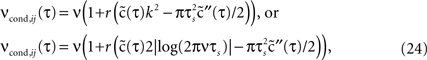
where  . Equation 24 shows that weak spike correlations are generally firing rate dependent and directly reflect the structure of input correlations C(τ). Figure 5
A shows three examples of voltage correlations which have the same τs, but different functional form. All three functional dependencies are reflected in the cross conditional firing rate νcond,ij, but result in markedly different shapes of auto conditional rate νcond(τ) (Figures 5
A,B). In the next section we study how the functional choice of C(τ) affects the correlation coefficient.
. Equation 24 shows that weak spike correlations are generally firing rate dependent and directly reflect the structure of input correlations C(τ). Figure 5
A shows three examples of voltage correlations which have the same τs, but different functional form. All three functional dependencies are reflected in the cross conditional firing rate νcond,ij, but result in markedly different shapes of auto conditional rate νcond(τ) (Figures 5
A,B). In the next section we study how the functional choice of C(τ) affects the correlation coefficient.Count correlations across spike trains
We now use the spike correlation function obtained above to study the pairwise count covariance.
which allows to obtain the correlation coefficient for a weakly correlated pair of neurons:
This offers the opportunity to study how changes in the input structure affect spike count correlations. Figure 5
shows that correlation coefficient ρij depends on both bin size T and the functional form of input correlation function C(τ). Figure 5
C illustrates that different functional form of underlying membrane potential correlations can lead to a strikingly different dependence of ρij on the bin size. After an initial increase for all three voltage correlation functions, correlation coefficient continues increasing slowly for C1, remains at the same level for C2, but decreases dramatically for C3. This latter type of behavior was not observed in previous studies of LIF models (de la Rocha et al. (2007)
, Suppl.), which focused on the analytically accessible choice of white noise currents and reported a monotonously increasing correlation coefficient in the limit of large T. Below we will further consider how dependence of ρij on T is influenced by the choice of the form of voltage correlations C(τ). We will show that some voltage correlation functions can lead to vanishing correlation coefficients in the limit of large bin size T.
Vanishing count covariance in the presence of cross correlations
Count covariances and correlation coefficients rely on the integral of the spike correlation function (Eqs 3 and 7). In cortical neurons, the spike correlation functions can exhibit oscillations and significant undershoots in addition to a correlation peak (Lampl et al., 1999
; Galan et al., 2006
), this may alter the correlation coefficients and their dependence on bin size T. In the weak correlation regime we obtained an analytic expression for νcond,ij(τ) (Eqs 24 and 26). This allows us to explore analytically how a change in the functional choice of voltage correlations will influence count correlations. To qualify as a reliable measure of synchrony, count cross correlations between two neurons should reflect primarily correlation strength and be independent of the functional form of input correlations. Our framework offers the possibility to test this hypothesis and explore whether previously reported finite correlation coefficients obtained for LIF model using white noise approximation (Shea-Brown et al., 2008
) can be generalized to a larger class of input correlations.
Here we consider spike correlations generated by a voltage correlation function with a substantial undershoot (e.g., as in Figure 1E in Lampl et al., 1999
). For illustration, we could use any voltage correlation function with a large undershoot and vanishing long-timescale variability ( ). Besides variance and correlation time, the variability as quantified by
  is an important characteristic of every noise process. For analytical tractability we chose the voltage correlation function C3(τ) as the normalized second derivative of the function
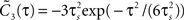
). Besides variance and correlation time, the variability as quantified by is an important characteristic of every noise process. For analytical tractability we chose the voltage correlation function C3(τ) as the normalized second derivative of the function 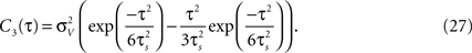
Defined this way, the correlation time of C3(τ) is τs and  , which is equivalent to vanishing spectral power for zero frequency. Figure 5
illustrates functional form of C3(τ) and the corresponding spike cross and auto correlations. The functional form of C3(τ) fulfills
, which is equivalent to vanishing spectral power for zero frequency. Figure 5
illustrates functional form of C3(τ) and the corresponding spike cross and auto correlations. The functional form of C3(τ) fulfills  . This leads to a vanishing count covariance and spike correlation coefficient for T >> τs (Eq. 26):
, which is equivalent to vanishing spectral power for zero frequency. Figure 5
illustrates functional form of C3(τ) and the corresponding spike cross and auto correlations. The functional form of C3(τ) fulfills . This leads to a vanishing count covariance and spike correlation coefficient for T >> τs (Eq. 26):
We note that the correlation coefficients and count covariances calculated for this functional form of input correlations can be arbitrarily small if T >> τs. This means that the absence of long-timescale variability in the inputs ( ) is equivalent to an absence of long-timescale co-variability in the spike counts. Notably, despite vanishing cross covariance, the variability of the single spike train is maintained and count variance of the single spike train (Eq. 8) is finite for C3(τ) in infinite time bins. Equation 28 implies that experimental correlation coefficients calculated for large time bins are most susceptible to the influence of temporal structure of correlations, and experimental studies focusing on large bin sizes [e.g., T = 192 ms (Greenberg et al., 2008
) or T = 2 s (Zohary et al., 1994
)] could potentially underestimate the correlation strength. For the important regime of low firing rates (Greenberg et al., 2008
), where the reset has little influence on the following spike, the threshold model and the LIF model can be expected to yield equivalent results. In this case, Eq. 28 and Figure 5
suggest that finite correlation coefficients, which are increasing with bin size T as reported for the LIF model (de la Rocha et al., 2007
) might be limited to the subset of input correlation functions without sizable undershoots. To obtain finite count cross correlations, the voltage correlation functions need to fulfill
) is equivalent to an absence of long-timescale co-variability in the spike counts. Notably, despite vanishing cross covariance, the variability of the single spike train is maintained and count variance of the single spike train (Eq. 8) is finite for C3(τ) in infinite time bins. Equation 28 implies that experimental correlation coefficients calculated for large time bins are most susceptible to the influence of temporal structure of correlations, and experimental studies focusing on large bin sizes [e.g., T = 192 ms (Greenberg et al., 2008
) or T = 2 s (Zohary et al., 1994
)] could potentially underestimate the correlation strength. For the important regime of low firing rates (Greenberg et al., 2008
), where the reset has little influence on the following spike, the threshold model and the LIF model can be expected to yield equivalent results. In this case, Eq. 28 and Figure 5
suggest that finite correlation coefficients, which are increasing with bin size T as reported for the LIF model (de la Rocha et al., 2007
) might be limited to the subset of input correlation functions without sizable undershoots. To obtain finite count cross correlations, the voltage correlation functions need to fulfill  , as C1(τ),C2(τ) in Figure 5
do.
, as C1(τ),C2(τ) in Figure 5
do.
) is equivalent to an absence of long-timescale co-variability in the spike counts. Notably, despite vanishing cross covariance, the variability of the single spike train is maintained and count variance of the single spike train (Eq. 8) is finite for C3(τ) in infinite time bins. Equation 28 implies that experimental correlation coefficients calculated for large time bins are most susceptible to the influence of temporal structure of correlations, and experimental studies focusing on large bin sizes [e.g., T = 192 ms (Greenberg et al., 2008
) or T = 2 s (Zohary et al., 1994
)] could potentially underestimate the correlation strength. For the important regime of low firing rates (Greenberg et al., 2008
), where the reset has little influence on the following spike, the threshold model and the LIF model can be expected to yield equivalent results. In this case, Eq. 28 and Figure 5
suggest that finite correlation coefficients, which are increasing with bin size T as reported for the LIF model (de la Rocha et al., 2007
) might be limited to the subset of input correlation functions without sizable undershoots. To obtain finite count cross correlations, the voltage correlation functions need to fulfill , as C1(τ),C2(τ) in Figure 5
do.Notably, spike count correlations of cortical neurons in vivo can decrease or increase as the length of the time bin increases (Averbeck and Lee, 2003
; Smith and Kohn, 2008
). These results are consistent with our findings (Figure 5
C). Thus, in contrast to the correlation coefficients computed for small T which are independent of C(τ) (Eqs 9 and 19), the count correlations computed for T ≥ τs are a potentially unreliable measure of synchrony.
Unambiguous and concise measures of spike correlations are needed to quantify and decode neuronal activity (Abbott and Dayan, 1999
; Greenberg et al., 2008
; Krumin and Shoham, 2009
). Pairwise spike count correlations are frequently used to describe interneuronal correlations (Averbeck and Lee, 2003
; Kass and Ventura, 2006
; Greenberg et al., 2008
) and many population models are based on these measures (Schneidman et al., 2006
; Shlens et al., 2006
; Roudi et al., 2009
). However, quantitative determinants of count correlations so far remained largely elusive. Here, we used a simple statistical model framework based on the threshold crossings and the flexible choice of temporal input structure to study the signatures of input correlations in count correlations. In general, the details of the spike generating model can have a strong effect on spike correlations, f.e. depending on the dynamical regime, two quadratic integrate and fire neurons or two LIF neurons can be more strongly correlated (Vilela and Lindner, 2009
). Notably, we found that our statistical framework can replicate many important aspects of neuronal correlations, e.g., nonlinear dependence of spike correlations on the input correlation strength (Binder and Powers, 2001
) (Eq. 19), firing rate dependence of weak spike correlations (Svirskis and Hounsgaard, 2003
; de la Rocha et al., 2007
) (Eq. 20), and independence of spike reliability of the threshold (Mainen and Sejnowski, 1995
) (Eq. 21). Furthermore, spike correlations derived here are consistent with many recent results in the commonly used LIF model, e.g., firing rate dependence of weak cross correlations (de la Rocha et al., 2007
; Shea-Brown et al., 2008
) (Eqs 20 and 24), the influence of noise mean and variance on the firing rates and weak spike correlations (Brunel and Sergi, 1998
; de la Rocha et al., 2007
; Ostojic et al., 2009
) (Eqs 15, 20 and 24), or sublinear dependence of correlation coefficients on input strength (Moreno-Bote and Parga, 2006
; de la Rocha et al., 2007
) (Eq. 19, Figure 3
). While the analytical accessibility of the LIF model is limited by the technically demanding multi dimensional Fokker–Planck equations and provides solutions only in special limiting cases (Brunel and Sergi, 1998
; de la Rocha et al., 2007
; Shea-Brown et al., 2008
), the framework presented here allows for an analytical description of spike correlations.
Measurements of correlation coefficients under different experimental conditions often aim to compare the input correlation strength in pairs of neurons (Greenberg et al., 2008
; Mitchell et al., 2009
). But is a change in count correlations always indicative of a change in input correlations? The tractability of our framework revealed that spike count correlations can be a poor indicator of input synchrony for some cases of input correlations. Count correlations computed for time bins smaller than the intrinsic scale of temporal correlations could be independent of the functional form of input correlations but depend on the firing rate and input correlation strength. This suggests that a change in the correlation coefficient can be related to a change in the input correlation strength, if a firing rate change and a change of intrinsic time scale can be excluded. On the other hand, a change in correlation coefficients computed for large time bins is indicative of a change in input correlation strength only if a change in firing rate, time scale and functional form of input correlations can be excluded. Furthermore, count correlations computed for large time bins can either increase or decrease with increasing time bin or even vanish in a correlated pair. This seemingly contradictory behavior is consistent with the functional dependence of spike count correlations observed in cortical neurons (Averbeck and Lee, 2003
; Kass and Ventura, 2006
; Smith and Kohn, 2008
).
Our results suggest that emulating neuronal spike trains, building efficient population models or determining potential decoding algorithms requires the analysis of full spike correlation functions in order to compute unambiguous spike count correlations. In particular, spike count coefficients computed for time bins larger than intrinsic timescale of correlations can be an ambiguous estimate of input cross correlations in a neuronal population with potentially heterogeneous distribution of input structures. Furthermore, the details of the spike generation model can be very influential for the transfer of current correlations to spike correlations, and the analytical results obtained here could facilitate quantitative comparisons between different types of models and between models and real neurons, by providing a maximally tractable limiting case for future studies.
The authors declare that the research was conducted in the absence of any commercial or financial relationships that could be construed as a potential conflict of interest.
We wish to thank M. Gutnick, I. Fleidervich, S. Ostojic and A. Malyshev for fruitful discussions and the Bundesministerium für Bildung und Forschung (#01GQ0430,#01GQ07113), Goettingen Graduate School for Neurosciences and Molecular Biosciences, German-Israeli Foundation (#I-906-17.1/2006), University of Connecticut and the Max Planck Society for financial support.