1
Department of Mathematics, University of Reading, Reading, UK
2
School of Psychology and Clinical Language Sciences, University of Reading, Reading, UK
Inverse problems in computational neuroscience comprise the determination of synaptic weight matrices or kernels for neural networks or neural fields respectively. Here, we reduce multi-dimensional inverse problems to inverse problems in lower dimensions which can be solved in an easier way or even explicitly through kernel construction. In particular, we discuss a range of embedding techniques and analyze their properties. We study the Amari equation as a particular example of a neural field theory. We obtain a solution of the full 2D or 3D problem by embedding 0D or 1D kernels into the domain of the Amari equation using a suitable path parametrization and basis transformations. Pulses are interconnected at branching points via path gluing. As instructive examples we construct logical gates, such as the persistent XOR and binary addition in neural fields. In addition, we compare results of inversion by dimensional reduction with a recently proposed global inversion scheme for neural fields based on Tikhonov–Hebbian learning. The results show that stable construction of complex distributed processes is possible via neural field dynamics. This is an important first step to study the properties of such constructions and to analyze natural or artificial realizations of neural field architectures.
Neural field theories are continuum approximations for high-dimensional neural networks (Griffith, 1963
; Wilson and Cowan, 1973
; Amari, 1977
; Ermentrout and McLeod, 1993
; Jirsa and Haken, 1996
; Robinson et al., 2001
; beim Graben, 2008
). In a rather general form (Wilson and Cowan, 1973
; beim Graben, 2008
), the neural field equation can be given by an integro-differential equation
where u(x,t) describes the spatio-temporal activity of the neural tissue at position x ∈ D and at time t ∈ ℝ. The spatial domain D ⊂ ℝn with n = 1, 2 or 3 are typical dimensions in applications. The function τ(x) describes a spatially dependent time constant for neural activation, while the integral kernel w(x, x′) indicates the synaptic connectivity and strength between sites x and x′ in the neural tissue. The temporal kernel G(t) is the postsynaptic impulse response function, and c the neural propagation velocity. Finally, f is a sigmoidal activation function describing the conversion of membrane potential u(x,t) to spike rates at the axon hillock.
The interpretation of Eq. 1 is therefore as follows: The left-hand side describes the intrinsic decay dynamics of neural activation u(x,t) with time constant τ(x), whereas the right-hand side accounts for the net input to u(x,t) via synaptic connections. The spatial integral generalizes the usual weighted summation of activity delivered to neurons at x from neurons at x′. On the other hand, the temporal convolution models summation of postsynaptic potentials over time together with axonal propagation delay.
Note that even more general versions of neural field equations contain a distribution of propagation velocities ρ(c), instead of a fixed velocity c. Accordingly, they involve a third integration over dc at the r.h.s. of the neural field equation (Nunez, 1995
; Hutt and Atay, 2006
). Hutt and Atay (2006)
were able to demonstrate that the variance of the velocity distribution affects the frequency of bifurcating periodic solutions and the phase speed of travelling waves. More interestingly, they discovered that the introduction of velocity distributions lead to the maximization of travelling front speed.
Equation 1 can be substantially simplified by assuming spatial homogeneity of time constants, τ(x) = τ, infinite signal propagation c = ∞ and instantaneous postsynaptic processing, G(t) = δ(t). As a result, one obtains the Amari equation (Amari, 1977
) with inhomogeneous kernel in the form

where the nonlinear activation function f is given as

with constants gain β > 0, and threshold η ∈ ℝ. The Amari equation characterizes a simple neural field theory and serves as a basic model to discuss and implement neural field architectures and neural field phenomena. We shall restrict our attention to basic important phenomena here.
Interpreting the domain D ⊂ ℝn of the Amari equation 2 not as a physical substrate realized by actual biological neurons, but rather as an abstract feature space for computational purposes, one also speaks about dynamic field theory (Thelen et al., 2001
; Erlhagen and Schöner, 2002
).
The description of logical reasoning and digital computation by means of neural network architectures is at the focus of research since the pioneering work of McCulloch and Pitts in the 1940s (McCulloch and Pitts, 1943
) and has been investigated, e.g. by Balkenius and Gärdenfors (1991)
, Mizraji and Lin (2001)
, Blutner (2004)
, in the sequel. In the framework of neural or dynamic field theory, Wennekers (2006
, 2007)
used operational cell assemblies as such a computing paradigm. Here, we will study another approach to this goal on the basis of neural field theory. The general task of implementing cognitive or logical processes can be described by a hierarchy of three tiers (compare beim Graben and Potthast 2009
). The top level is the cognitive level where cognitive processes are modelled with tools from symbolic logic. The second level is the representation level, which contains fields representing the cognitive processes in terms of wave fields, states and field dynamics. The third and bottom level is a neural field level where neural fields and neural kernels implement the dynamics of the representation level.
When the dynamical fields in the representation level are given, we need to solve the inverse problem of constructing appropriate neural kernels implementing the dynamics, compare beim Graben and Potthast (2009)
, Potthast and beim Graben (in press)
. Usually, for more complex tasks of cognition these are high-dimensional inverse problems, which exhibit significant computational cost as well as high degree of instability or ill-posedness.
In this work, we mainly address two tasks. The first task is to provide a method for constructing neural field kernels for more complex cognitive tasks which is less computationally expensive and less ill-posed than the earlier approaches (beim Graben and Potthast, 2009
; Potthast and beim Graben, in press)
.
Usually the term problem reduction is used when a difficult problem is solved by reducing it to easier problems. In this sense the term dimensional reduction describes the process from an inverse problems perspective, since we reduce the multi-dimensional inverse problems to the solution of low-dimensional tasks.
We will solve the problem by constructing low-dimensional embeddings of neural kernels into higher-dimensional neural domains. In particular, we will describe zero-dimensional and one-dimensional embeddings into two- (or possibly three-dimensional) neural tissue. This is employed for the construction of paths for neural pulses, for gluing different path patches together, for designing AND, OR and XOR gates as well as delay gates which can be used for synchronization of neural pulses.
The second task is to study more general Hilbert-space based implementations of cognitive processes on the basis of neural field theory. Neural field equations such as Eq. 1 or the Amari equation 2 are often transformed into partial differential equations for further analysis (Jirsa and Haken 1997
; Coombes et al., 2003
). This, however, restricts the synaptic weight kernels considerably, by presupposing local interactions. On the other hand, generating and understanding non-local distributed cognitive dynamics with complex logical decisions is of high interest both for controlling and constructing neural computing architectures as well as for analyzing natural phenomena in biological neural systems (Jirsa and Kelso 2000
; Bressloff and Cowan 2002
). We will realize this dynamics by using basis transformations from special embedded dynamics, in particular we employ basis transformations from simple localized basis functions onto distributed global functions on our neural domain which are realized as vectors with random components.
We will realize some generic logical tasks like AND, OR, XOR and more complex tasks like binary addition with three binary inputs and a gating pulse on the basis of neural field theory. To this end we first design the processes on an abstract logical level and then describe different realizations and embeddings in the framework of a neural field theory.
In Section “Solving Inverse Neural Field Problems” we provide an introduction into main tools from the theory of inverse problems which can be used to solve low or high-dimensional inverse problems. We will use the tools in subsequent sections for constructing low-dimensional neural field kernels for prescribed neural dynamics. Section “Embedding One-dimensional Processes into 2d or 3d Neural Tissue” is the first key section to describe embedding techniques and to construct basis kernels for elementary logical functions based on a neural field environment. Section “Embedding 0D Logic into Neural Tissue” serves to describe a zero-dimensional version of the embedding theory. This can also be viewed as an embedding of a classical neural network into a neural field environment. An abstract view based on Hilbert space theory is provided in Section “An Abstract View and Basis Transformations”. We discuss Hilbert space based dynamics and basis transformations in the framework of Amari neural fields with a particular focus on the stable construction of global neural dynamics. This leads to a distributed non-local logical dynamics, which is described and implemented. Numerical examples for each of the above sections are provided.
This section serves as summary and introduction into solving inverse problems in the framework of the Amari equation 2 as carried out by beim Graben and Potthast (2009)
, Potthast and beim Graben (in press) and Potthast and beim Graben (in press)
. It will be employed many times for the one-dimensional pulse construction in the following sections.
We prescribe one or several complete time-dependent patterns vξ(x, t), ξ = 1,…,n for x ∈ D, t ≥ 0 with some domain D ⊂ ℝp. For our further discussion we assume that the nonlinear activation function f : ℝ → [0,1] is known. Then, we search for kernels w(x,y) for x, y ∈ D, such that the solutions of the Amari equation with initial conditions u(x, 0) = vξ(x, 0) satisfies u(x, t) = vξ(x, t) for x ∈ D, t ≥ 0, and ξ = 1,…,n.
As a first step, we transform Eq. 2 into a linear integral equation. Defining
and employing the integral operator

leads to a reformulation of the inverse problem into the equation

where here the kernel w(x,y), x,y ∈ D, of the linear integral operator W is unknown. Equation 7 is linear in the kernel w. It can be rewritten as

with

For every fixed x ∈ D we can rewrite Eq. 7 as

with
wx(y) = w(x,y), x,y ∈ D, ψξ,x(t) = ψξ(x,t), x ∈ D, t ≥ 0.
If φ is continuous in y and t, then for fixed x, Eq. 10 is a Fredholm integral equation of the first kind with continuous kernel φ. This equation is known to be ill-posed (Kress, 1989
), i.e. we do not have (a) existence or (b) uniqueness in general and even if we have uniqueness the solution does not depend in a (c) stable way on the right-hand side.
In order to cope with ill-posedness and instability, several regularization techniques have been proposed in the literature. Among them, Tikhonov regularization is a very general scheme which can be derived via three different approaches: (i) by a spectral approach, (ii) from matrix algebra, or (iii) as an optimization procedure for solving an ill-posed equation Vg = f. Clearly, a solution to the equation Vg = f can be searched by the minimization

where X denotes some appropriate Hilbert space X, for example the space L2(D) of square integrable functions on some domain D. The normal equations (compare Kress, 1999
) for the minimization problem are given by
V*Vg = V*f.
The operator V*V does not have a bounded inverse. Stabilization is reached by adding a small multiple of the identity operator I (Kress, 1999
), i.e. by solving

which corresponds to adding a stabilization term α|| g ||2 to the minimization (Eq. 11), leading to the third form of the Tikhonov regularization

The operator Eq. 12 is usually discretized by standard procedures and then leads to a matrix equation which can be solved either directly or by iterative methods (Kress, 1999
).
The Moore–Penrose pseudoinverse is given by the limit of the Tikhonov regularization for α → 0, i.e. it is

However, as discussed above this limit will lead to satisfactory reconstructions only for well-posed problems. For the above-mentioned ill-posed inverse problem we have to employ α > 0.
These techniques were applied to neural pulse construction problems by Potthast and beim Graben (in press)
, Potthast and beim Graben (in press) and beim Graben and Potthast (2009)
. In particular, the authors demonstrated the feasibility of regularized construction techniques for synaptic kernel construction. Properties of the solutions were investigated and the ill-posedness of the problem was proven and demonstrated by particular examples.
Challenges for multi-dimensional inverse problems. As a preparation to the next parts of this work here we discuss one major disadvantage of the above approach when more complex problems are addressed.
It is well-known that solving multi-dimensional inverse problems is a difficult and challenging task of current research (Colton and Kress, 1998
). In particular, it is well-known that in general the ill-posedness of an inverse problem increases if
I. we use higher discretizations for the simulations of the forward problem,
II. the dimension and complexity of the mapping under consideration increases.
The reason for this phenomenon in both cases is that the calculations take into account more singular values and singular functions. The singular values strongly decay and taking more singular values into account corresponds to larger instability.
For cognitive neuroscience this means that both increasing the dimension and complexity of the simulated dynamics as well as enhancing the simulation algorithms by higher discretization will cause more severe instabilities for kernel construction problems. In addition, the computational costs are strongly dependent on the size of the problem under consideration, measured in terms of
a. the dimension of the neural domain,
b. the complexity of the dynamics,
c. the number of time discretization points,
d. the spatial discretization of the problem,
where c) and d) usually depend to some extent on a) and b), for example discretizations of a multi-dimensional problem needs much more discretization points than discretization of a one-dimensional problem.
Here, the size and condition number of the matrix Φ defined in Eq. 9 will strongly increase with the number of time-discretization steps. A detailed discussion of these effects can be found in Potthast and beim Graben (in press) and Potthast and beim Graben (in press)
. Yet the above works do not propose any approach to resolve the problems. They focus on the study of simple problems with basic tools from the theory of inverse problems. Our goal here is to introduce a computational technique which resolves the issue by use of embedding techniques. Our approach is related to similar approaches such as operational cell assemblies and continuous attractor networks (Thelen et al., 2001
; Erlhagen and Schöner, 2002
; Wennekers, 2006
, 2007) and we expect that the algorithms developed here can be employed to such approaches as well. The techniques allow stable and efficient solutions to complex and distributed neural modelling problems, we expect it to be an important step towards addressing more realistic questions of cognitive dynamics.
The approach in this work is to solve low-dimensional inverse problems with mild or no instability and to embed the solution into a higher-dimensional space. To this end we will first introduce an embedding technique in the next subsection and then apply it to plain pulse kernels and delay kernels. We show how different paths can be linked together leading to different types of branching point dynamics. Then, the construction of simple and more complex logical functions on the basis of embedded pulses is described.
The embedding technique here is independent of the technique which is used to calculate the kernels which are embedded. We will flexibly employ two different approaches to calculate low-dimensional kernels which are then embedded into higher-dimensional neural domains:
(1) analytical solutions/kernels given explicitly in closed form or
(2) kernels constructed numerically by solving the inverse problem of Section “Solving Inverse Neural Field Problems” on a low-dimensional set.
Path Embedding
Let  for
for  be a one-dimensional neural kernel. Our neural tissue is given by a domain D ⊂ ℝ2. We consider a path γ: [a,b] → D given by parametrization
  , and define its trace by
for be a one-dimensional neural kernel. Our neural tissue is given by a domain D ⊂ ℝ2. We consider a path γ: [a,b] → D given by parametrization , and define its trace by
We will use | · | for the Euclidean norm in ℝn and d(x,G) for the Euclidean distance of a point x to the domain or set G. We assume that
A1. γ is differentiable, i.e. for every point x ∈ Γ there is a tangential vector ζ(x) ∈ ℝ2 and a normal vector  ,
,
,A2. the size of the derivative Γ′(s) is strictly positive, i.e. there is a constant c1 such that |γ′(s)| ≥ c1 > 0 for all s ∈ [a,b],
A3. the mapping  is injective, i.e. there are no crossing points and double points of the path,
is injective, i.e. there are no crossing points and double points of the path,A4. the path embedding has sufficient distance to the boundaries of our neural tissue, i.e. d(Γ, ∂D) ≥ c2 > 0 with some sufficiently large constant c2.
The last condition is convenient to avoid technical overload of the arguments below. We are then prepared to define a tube of diameter ρ > 0 around a path Γ by

where d denotes the distance from x to Γ. If ρ is sufficiently small, the tube Γρ can also be defined as the set

In this case, for x ∈ Γρ there is a unique pair of parameters (s,r) = T(x) such that x = γ(s) + rv[γ(s)]. We use the abbreviation γρ(s,r): = γ(s) + rv[γ(s)] for s ∈ [a,b] and r ∈ [−ρ, ρ].
Definition 3.1. (Kernel Embedding) For ρ sufficiently small as in Eq. 17 depending on c2 and Γ we define the embedding of  into D by
into D by
An example of such a kernel embedding is shown in Figure 1
.
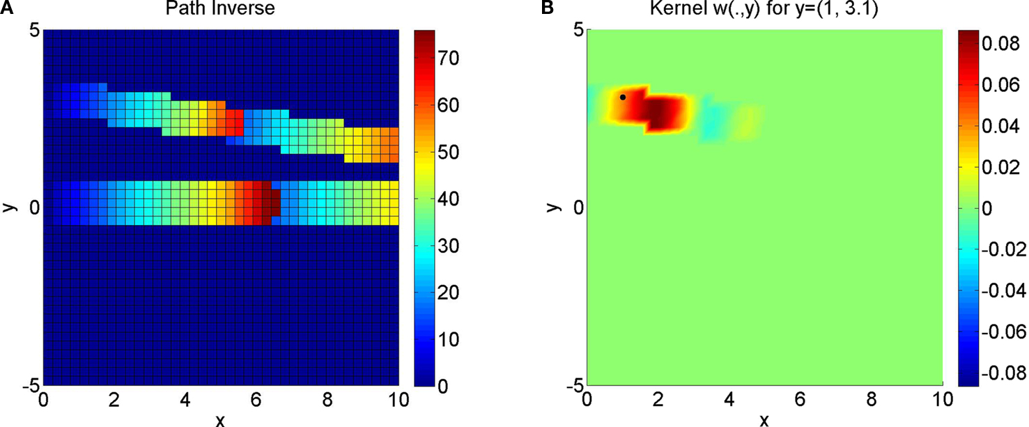
Figure 1. The image (A) shows several path embeddings, where for a point x ∈ D in the neural tissue D we visualize the index of the path vector Γ which is mapped onto x. The colour in (A) shows the parameter of a particular path. Where red overlaps light blue, two paths patches are glued together. The embedded kernel (calculated by a Tikhonov–Hebbian approach described in Section “Solving Inverse Neural Field Problems”) for the first of these path and a point y = (2.4276, 2.5724) is shown in image (B), illustrating the embedded kernel (Eq. 18). Here, the neuron located at the black point is exciting the red area and inhibiting blue areas.
We later study the processing of pulses similar to the work shown in beim Graben and Potthast (2009)
, Potthast and beim Graben (in press) and Potthast and beim Graben (in press)
. In particular, later we use Gaussian pulses

with σ > 0 and speed c > 0. With the embedded kernel under the conditions A1–A4 we will obtain a two-dimensional pulse which is analogous to the one-dimensional pulse dynamics, but now follows the prescribed path Γ or tube Γρ, respectively.
The construction of the two-dimensional kernels (Eq. 18) is carried out such that the kernel is the same for all points in a tube which are on a line

This also leads to an equivalence of the neural dynamics generated by the one-dimensional kernel and the two-dimensional embedded kernel (18).
We call a function u0 embedded into Γρ, if it is constant on lines L(x) defined by Eq. 20 for all x ∈ Γ. In this case u0 corresponds to a one-dimensional function  defined on the parametrization interval [a,b] of Γ such that u0 is the embedded version of
  .
.
defined on the parametrization interval [a,b] of Γ such that u0 is the embedded version of .Theorem 3.2. Consider a path embedding Γ which satisfies A1–A4 and let the initial value u0 be an embedded function from  according to Definition 3.1. Then, the dynamics for the embedded kernel w with initial value u0 on Γ and the dynamics of the one-dimensional kernel
  with initial values
  are equivalent, i.e. the diagram
according to Definition 3.1. Then, the dynamics for the embedded kernel w with initial value u0 on Γ and the dynamics of the one-dimensional kernel with initial values are equivalent, i.e. the diagram
is commutative, i.e. we can either first carry out the one-dimensional dynamics and then embed the resulting dynamical field or we can first embed the initial condition and then carry out the embedded two-dimensional dynamics.
Proof. The proof is a direct consequence of the particular embedding technique. The two-dimensional dynamics includes the two-dimensional integral with the excitation or forcing term

We evaluate this integral for points x = γρ(s,r), s ∈ [a,b] and r ∈ [−ρ,ρ] in the tube Γρ as follows. Substituting  for
for  we calculate
for we calculate
which is the r.h.s of the one-dimensional Amari equation, thereby reducing the two-dimensional dynamics to a one-dimensionalcase. □
Plain Pulses
The goal of this section is to set up simple kernels which lead to one-dimensional travelling neural pulses v(x,t) for x ∈ ℝ and t ∈ ℝ on the real line ℝ. The generation of neural pulses by homogeneous kernels has been intensely studied, compare Amari (1977)
, Ermentrout and McLeod (1993)
, Coombes et al. (2003)
, Potthast and beim Graben (in press)
. Here, we will either provide an analytical solution or employ the Tikhonov–Hebbian approach described in Section “Solving Inverse Neural Field Problems”. We apply the techniques of the preceding Section “Solving Inverse Neural Field Problems” to construct a kernel to generate the dynamics of a pulse of the form (Eq. 19).
Alternatively, we may obtain stable pulse-like solutions as follows. We define a one-dimensional kernel with backward Gaussian inhibition and forward Gaussian excitation by explicit analytical construction

with constants c+, c− > 0 and s0 > 0. For an appropriate choice of constants c± and s0 by  and initial conditions by
and initial conditions by
we obtain travelling pulses in one dimension for the Amari field equation 2. This can be verified by numerical simulation or, for particular cases, by elementary arguments. We skip the details of the arguments since they work along the lines of Potthast and beim Graben (in press)
.
Delay Gates
Delay gates are logical elements which synchronize pulses travelling with different speed or which have to travel over a different distance. A delay gate keeps a pulse active over some time interval, such that pulses arriving earlier and pulses arriving later as input into some logical element lead to simultaneous excitation of the input areas. Delay gates are neural field implementations of delay lines for neural networks (Hertz et al., 1991
).
Here, we will construct delay gates which realize an excitation at the exit of the gate as soon as a pulse enters the gate area and keep the excitation at the exit constant while the pulse is passing through the delay gate. This synchronizes pulses over a time window of the travel time of a pulse through the gate.
In more detail, a delay gate is a kernel w(x,y) defined on an interval [a,b] ⊂ ℝ such that any pulse with sufficiently large active support entering the interval [a,b] leads to an excitation of the neural field in a neighbourhood of sufficient size of b as long as the pulse is travelling through the interval I[a,b].
The construction of delay gates can be done by solving neural inverse problems or by direct construction. Here, we employ the inversion technique of Section “Solving Inverse Neural Field Problems”. A delay gate is obtained by solving the inverse problem (Eqs. 7–10) with training pulse given by

for t ∈ [0,T], where  denotes the sigmoidal activation function defined in Eq. 3. The constants η0 and β control the time delay after which the excitation at the exit point of the delay gate becomes active.
denotes the sigmoidal activation function defined in Eq. 3. The constants η0 and β control the time delay after which the excitation at the exit point of the delay gate becomes active.Without an initial field the field in the gate will just be 0. If a pulse enters the gate, it corresponds to the initial training pattern (Eq. 28) and excites the complete path of the training pattern, which leads to an excitation of the exit pulse after a time interval η0 which is kept constant for the duration of pulse travel through the gate.
We numerically demonstrate a delay gate in Figure 2
. The figure shows one time slice of the dynamics for two different pulses. In the upper image the pulse entered the gate earlier than in the lower image, both pulses simultaneously excite a pulse at the exit area around coordinate x = 10.
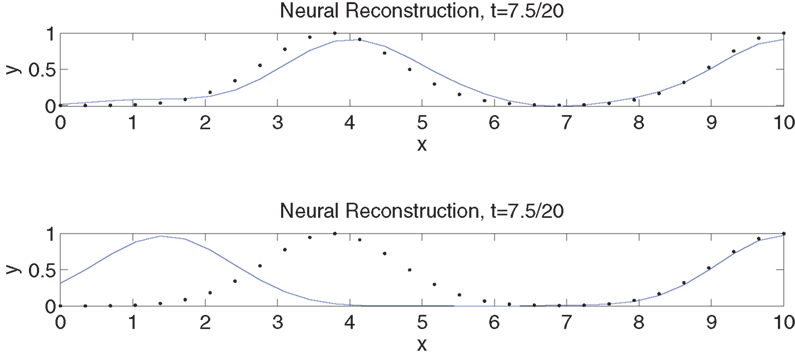
Figure 2. We show the time-slice of a delay gate dynamics as described in Section “Embedding One-dimensional Processes into 2d or 3d Neural Tissue”. Here, the delay gate is the complete interval between x = 0 and 10. In the upper graphics the pulse (blue line) entered the delay gate earlier than in the second image. Both pulses excite the exit area of the gate simultaneously. The dotted curve shows the original training patterns. For the generation of the neural kernel we used the inversion technique of Section “Solving Inverse Neural Field Problems”.
Branching Points and Gluing Paths Together
We employ the following technique for branching points and gluing paths together. As a preparation we note that the kernel for a plain path provides a direction for this path. A pulse has an entry point at one side of the tube and an exit point at the other. Pulses will only propagate from the entry point to the exit point. A pulse entering an exit point will die.
We speak of gluing together two or more paths at a point when we overlap an exit area with one or several entry areas or an entry area with several exit areas of different paths. We have employed the following elementary assumption for our constructions:
A5. We assume that there is a positive distance between any two tubes given by two paths, except for overlap in the case where we glue together two or more paths at a branching point.
The following points describe the gluing process in more detail:
1. If we want to glue together two paths Γ1 and Γ2, they need to be embedded with sufficient overlap such that a pulse exciting the tube Γ1,ρ (which does not have neural connections from the interior of Γ1,ρ into the exterior of Γ1,ρ) excites the pulse travelling through the tube Γ2,ρ. Here, we used an overlap as described in A5. containing a ball of radius ρ.
2. Consider the embedding w1 for path Γ1 and the embedding w2 for path Γ2, with overlap constructed as demanded in Item 4. Then a glued pulse is constructed by

3. According to the embedding technique for kernels the intersection of the support of w1 and w2 is a subset of the path overlap, i.e. where both x and y are in Γ1 ∩ Γ2. For most kernels considered in this work the kernels do not have a significant size when x and y are very close to each other, such that the summation (Eq. 29) does not disturb the pulse behaviour significantly in Γ1 ∩ Γ2.
We demonstrate the gluing of paths in Figure 1
. Our numerical tests with travelling pulses below confirm the above arguments and show that we can glue paths together without difficulty. The technique has been employed for the example of binary addition in Section “An Abstract View and Basis Transformations”, compare also Figure 5
.
Branching and OR Logic. Branching points are points where more than two pulses are glued together. Given three paths Γ1,Γ2 and Γ3 we construct a branching point from embeddings w1,…,w3 which have some overlap around the point p ∈ D by

Branching points are natural realizations of logical structures. As an example consider Figure 3
. The figure shows path embeddings as blue lines between the black points. Three branching points can be identified.
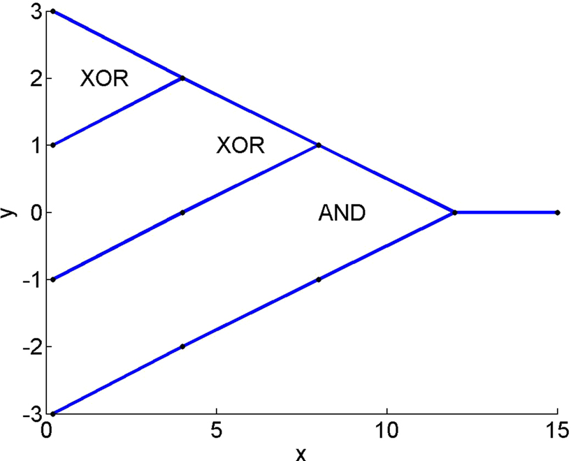
Figure 3. A logical design for a gated binary addition, where here the last digit as defined in Eq. 35 is calculated.
Here, as a simple example and first step towards more complicated logic we formulate logical OR and multiplexer elements via branching points. A pulse corresponds to the logical input true or 1. No pulse corresponds to false or 0.
Algorithm 3.3. OR Logic, Multiplexer Branching points where w1 and w2 are incoming and w3 is outgoing implement the classical OR logic in the sense that a pulse is transmitted through Γ3 if either a pulse enters the branching point through Γ1 or through Γ2 or both Γ1 and Γ2.
Branching points where w1 is incoming and w2, w3 are outgoing implement a multiplexer logic in the sense that a pulse entering the branching point will be transmitted into both w2 and w3.
Logical Elements
Further logical elements are now constructed using embedded pulses, branching points and additional inhibition elements.
An inhibition element is a neural kernel wi defined on two subsets V1 ⊂ Γ1,ρ and V2 ⊂ Γ2,ρ such that
An inhibition element establishes an inhibition which is activated by a pulse travelling through V1 and is applied to any field in V2.
We are now prepared to define all standard logical elements within the neural field environment. Here, we pick selected examples.
XOR Logic. Consider three points pin,1, pin,2 and pout ∈ D in a neural tissue. We consider pin,1 and pin,2 as input nodes and pout as output node for logical processing, i.e. we expect input pulses in a neighbourhood Bρ(pin,1) or Bρ(pin,2) of these points as input. The output will be a field activation u which is above the threshold η on Bρ(pout). We need to assume that

where d(p, q) denotes the Euclidean distance between points p and q in D.
1. Let wplain,ξ be an embedded kernel for a plain pulse from pin,ξ to pout along a path Γξ, where the tube Γξ,ρ has distance larger than ρ to the point pin,η for η ≠ ξ, η, ξ = 1,2. We assume that the tubes Γ1,ρ and Γ2,ρ intersect only on the exit area around pout.
2. Let wi,ξ be an inhibition kernel for the subsets Γξ,ρ\V and Γη,ρ\V with V: = Γξ,ρ ∩ Γη,ρ for ξ ≠ η, ξ, η = 1,2, i.e. wi,ξ establishes an inhibition of fields in Γη,ρ \ V when a pulse in the tube area Γξ,ρ\V is active.
If the constants are chosen appropriately, the above setting realizes a logical XOR functionality.
Algorithm 3.4. XOR Logic. The kernel
establishes a XOR functionality for pulses entering the tubes Γ1 and Γ2 connecting pin,1 and pin,2 with pout. The functionality will be satisfied for pulses entering the paths Γ1 and Γ2 at any point and during the time window defined by the remaining travel time of a pulse through these paths.
We have numerically tested the above scheme independently and for realizing the binary addition logic described in Section “An Abstract View and Basis Transformations” and shown in Figure 5
, where traces of time-dependent travelling pulses are shown. The underlying logical structure is visualized in Figure 3
. We assume that an input excitation is given to the input nodes at (0,−1), (0,1) and (0,3), the node (0,−3) serves as a gating pulse to activate the complete logical gate. As before, a pulse corresponds to the logical input true or 1. No pulse corresponds to false or 0. The inhibition components lead to mutual inhibition between the pulses in the paths of the XOR elements.
Here we have combined analytical parts (the inhibition elements are explicitly prescribed) with results of the inversion of Section “Solving Inverse Neural Field Problems” for obtaining travelling pulses in the lines between the nodes. The elements are constructed in one dimension and then embedded into the two-dimensional neural domain by the embedding technique of Definition 3.1.
AND Logic. There are at least two basic options to realize the classical AND logic for pulses. The first option combines the OR logic given by Algorithm 3 with a damping of the kernels in the overlap of the exit point.
Algorithm 3.5. AND Logic I. Let wor be the kernel constructed in Algorithm 3 and V: = Γξ,ρ ∩ Γη,ρ. We define a damped kernel by
with damping factor cd ∈ (0,1). If the damping factor is chosen appropriately (depending on ρ and the kernel setup), then wand establishes the AND functionality for pulses entering Γ1 and Γ2. The time window for synchronization here is rather short, since both pulses need to arrive at ρout simultaneously. This can be enhanced by using delay gates in both of the tubes which are involved.
An alternative implementation of AND is provided by the following architecture, visualized in Figure 4
.
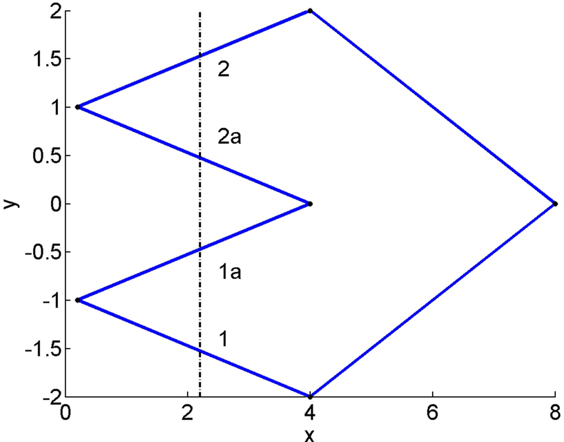
Figure 4. A structural design for a stable logical AND gate. The dashed line separates different parts of the logical paths for 1, 2, 1a and 2a where different inhibition effects are employed, details are introduced in the points 1–4 in Algorithm 3.6. Pulses enter at the nodes in (0,−1) and (0,1). The output node is at (8,0).
Algorithm 3.6. AND Logic II. We construct path embeddings as visualized in Figure 4
with the following path kernels and inhibitions:
1. From two input nodes we construct two paths each by a multiplexer branching point according to Algorithm 3.3. This leads to four paths labelled 1, 1a, 2 and 2a. We use the numbers as abbreviations for either paths or tubes.
2. We now apply inhibition from 1 to 2a and from 2 to 1a on the first half of the paths.
3. After that in the second half of the path we apply inhibition from 1a to 1 and from 2a to 2.
4. Then, we connect 1 and 2 to the endpoint by a simple OR gate.
The combination of the steps 1 to 4 generates a logical AND gate embedded into neural tissue.
To show the validity of the above setup we need to check four situations, with no pulses or with pulses entering in either pin,1, pin,2 or in both points. No pulse represents 0&0 = 0, which is clearly satisfied. Consider the situation 1&0. In this case we get pulses in 1 and 1a. Then 1a inhibits the pulse in 1 such that it dies and there is no output pulse, i.e. 1&0 = 0 is satisfied. The same logic applies to the pulses in 2 and 2a. Now, consider two pulses 1&1. Then first they split into four pulses 1, 1a, 2, 2a. Now we apply step 2, such that the pulses in 1a and 2a die by inhibition from 2 and 1. Then the remaining pulses in 1 and 2 go through and via the OR gate reach the final point pout, which establishes the logic 1&1 = 1.
The advantage of the AND logic of Algorithm 3.5 is that it is a very simple and natural implementation depending on the special size of the kernel w. The second implementation is much more independent of this size and much more stable with respect to strength variations of w. Both designs are implemented in a neural domain by the embedding techniques of Definition 3.1.
Binary Addition. Finally, we would like to show a more complex implementation of binary addition. Here, we have realized the addition of three binary numbers triggered by a gating pulse, i.e. we realize

The logical design is summarized in Figure 3
. The idea is that the pulses enter the neural domain at points (0,−1), (0,1) and (0,3), where we also added a gating pulse with entry at (0,−3). We will study different solutions of the realization of the above logical structure. The first solution is a pulse-based approach where the pulses are constructed in one dimension first on the basis of Section “Solving Inverse Neural Field Problems”. They are embedded into a two-dimensional neural domain, combined with inhibition elements, glued together at branching points or simple connection points. The second and third approach will be described in the following sections.
In Figure 5
we show the trace of the pulses – not their time-behaviour, i.e. we show all points red where the pulse is above the threshold at some point of time. The binary inputs are the first three input nodes on the left-hand side of the tissue, the output node is the centred node on the right-hand side.
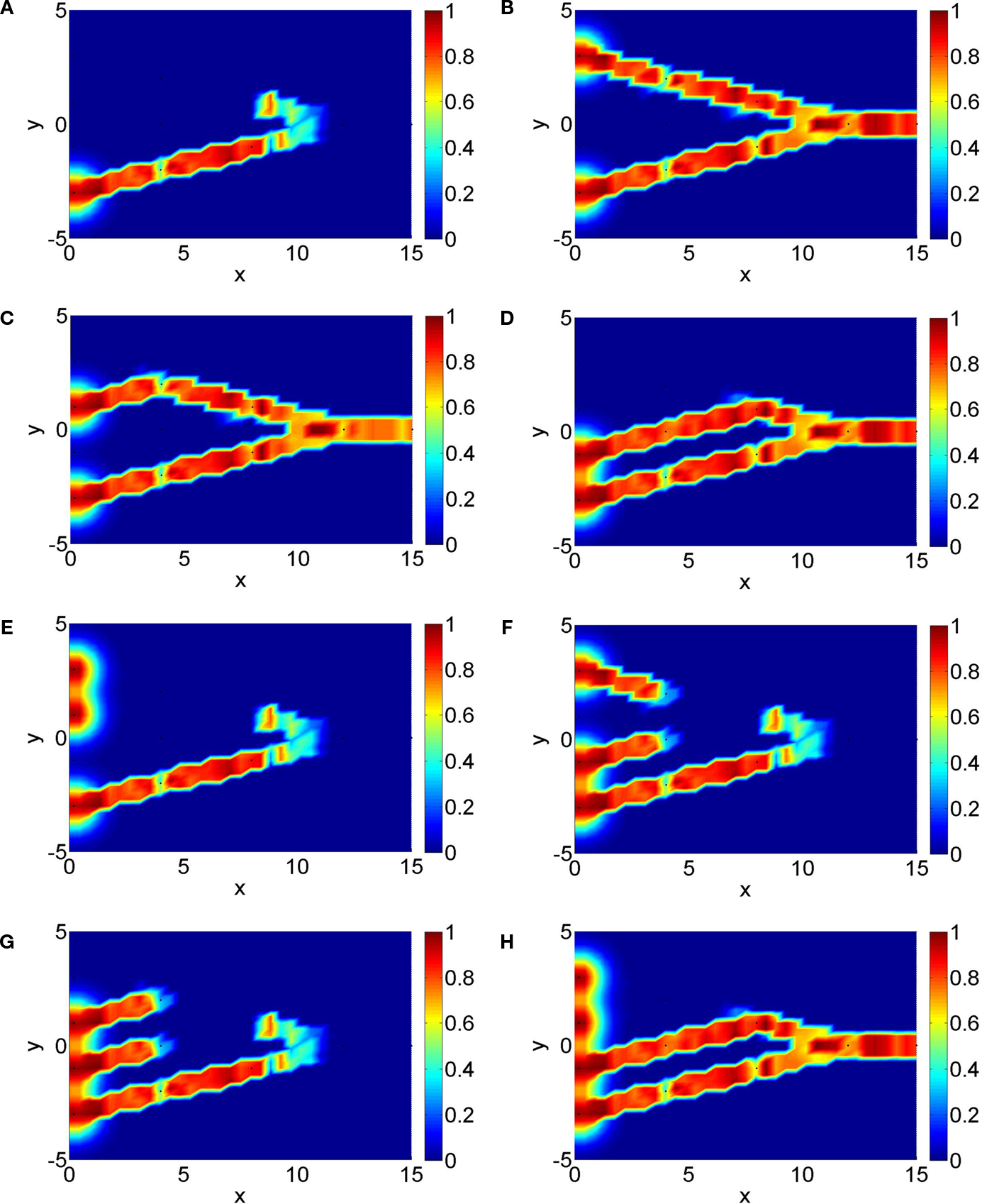
Figure 5. The images show the traces of neural pulses for the last binary digit of a gated binary addition logic (Eq.35a–h) corresponding to the panels A–H via the one-dimensional embedding technique in combination with low-dimensional inverse problems and analytical elements for the logical components.
Our approach here to a 0D embedding is the reduction of neural pulse dynamics. We consider the neural tissue D to be global in the sense that every point x can be influenced by a neural field at the point y ∈ D. But this means that we do not need to process an influence by a travelling pulse, but we can directly excite the corresponding areas in a non-local fashion.
In contrast to a path embedding, here we need only to embed two or more points with their neighbourhoods into the neural tissue to realize a logical function. Since a point is a zero-dimensional manifold, we call the embedding zero-dimensional (0D).
The implementation of such 0D embeddings reflects old issues of implementing logical functions in neural networks (Hertz et al., 1991
). For example, a logical XOR functionality cannot be implemented by directly linking two input nodes to the output node. We need to include at least two further points with their neighbourhoods.
With the neural field we have a highly integrated continuous auto-associative network in which we may embed classical neural network logic. But we also gain new options for these embeddings and the deep tools of mathematical analysis and functional analysis are available to investigate and control such embeddings. These further options will be explored in our final section, here we will provide more details on the 0D embedding.
Pulses. Zero-dimensional versions of pulses are direct excitations of the target areas within the neural tissue. To obtain a speed of pulse propagation comparable to the speed of elementary logical elements we have used a one-stop pulse realization, i.e. from an area around an input point pin we have first excited an auxiliary area around a point paux and then this area excites the target area around pout.
XOR Logic. For the XOR gate we have used a zero-dimensional logic with five points, two input points pin,1, pin,2, two auxiliary points paux,1, paux,2 and the output point pout. Excitation is taking place from pin,ξ to paux,ξ and from paux,ξ to pout for ξ = 1,2. Inhibition is realized from pin,ξ to paux,η with ξ = η, ξ, η = 1,2.
AND Logic. For the AND gate as for XOR we have used a zero-dimensional logic with six points, two input points pin,1, pin,2, three auxiliary points paux,1, paux,2, paux,3 and the output point, pout. Excitation is taking place from pin,ξ to paux,ξ for ξ = 1,2, from pin,ξ to paux,3 and from paux,ξ to pout for ξ = 1,2. Inhibition is realized from paux,3 to pout. Here, a single input in either pin,1 or pin,2 will excite either paux,1, paux,3 or paux,2,paux,3. Then the inhibition of paux,3 to pout will cancel the excitation if there are not two simultaneous excitations from paux,1 and paux,2.
In the results of Figure 6
the auxiliary points have been inserted into the path between the input and output nodes. As in Figure 5
here we show the trace of the pulse, not its time-behaviour, i.e. we show all points red where the pulse is above the threshold at some point of time.
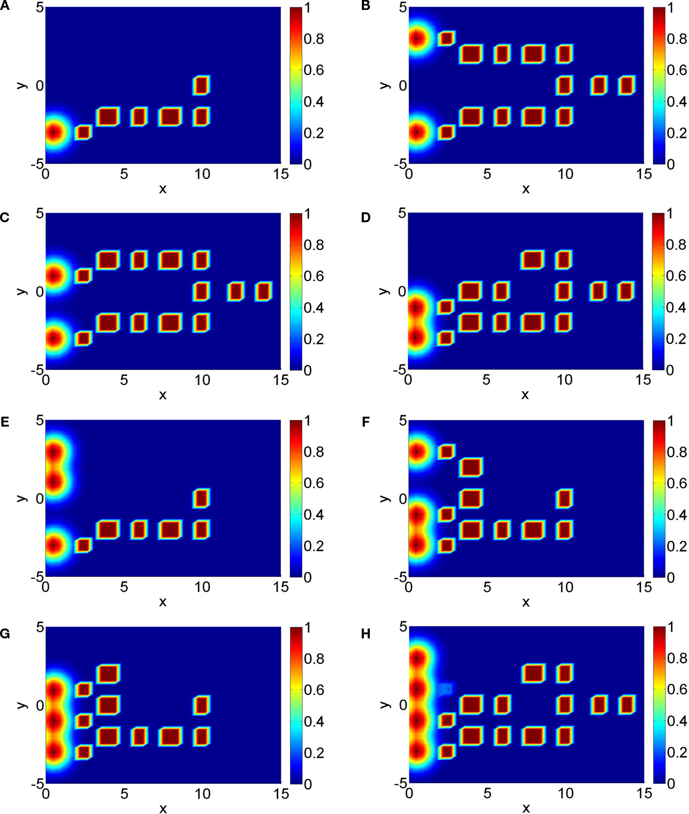
Figure 6. The images show the traces of neural pulses for the last binary digit of a gated binary addition logic (Eq. 35a–h) corresponding to the panels A–H via the zero-dimensional embedding technique with purely analytical elements for the logical components, compare Section “Embedding 0D Logic into Neural Tissue”.
Binary Addition. Finally, we have integrated the zero-dimensional embeddings into a binary addition logic. It is shown in the results of Figure 6
. The design is analogous to the one shown in Figure 3
.
The goal of this section is to formulate an abstract view into state space dynamics of logical computations. Logical dynamics is often regarded as processing from one logical state to another (Wennekers, 2006
, 2007
; beim Graben and Potthast, 2009
). Here, we will construct particular logical states and neural mappings from one state to another using the zero-dimensional embeddings from Section “Embedding 0D Logic into Neural Tissue” and Hilbert space basis transformations. Thus, we stably construct complex distributed state-space dynamics for neural processes.
Hilbert Space Dynamics
We aim to discuss a Hilbert space dynamical implementation of logical structures. Let X be some Hilbert space.
Definition 5.1. Let X be a Hilbert space and consider a parameterized mapping

with the property

for all t,s > 0. A mapping of the type (Eq. 36), (Eq. 37) establishes a Hilbert space dynamics.
Remark. Given an initial value u0 ∈ X, the dynamics St defines a time-dependent field

with the property

i.e. the operator Ss describes the change of the field ut from t to t + s. This is well-known as semi-group representation in the mathematical theory of dynamical systems (Anosov and Arnol’d, 1988
). Here, it establishes an abstract concept which is realized by the Amari neural field equation 2.
We can discretize the dynamics by considering

with some grid constant ht. Then, according to Eq. 37 the complete dynamics is given by iterating  .
.
.We consider elements  for k = 1,…,n and j = 1,…,m. Our goal here is the construction of particular dynamical systems which satisfies
for k = 1,…,n and j = 1,…,m. Our goal here is the construction of particular dynamical systems which satisfies
with initial values  for j = 1,…,m. For fixed j the sequence of points
  , k = 1,…,n is a realization of a particular part of logical inference.
for j = 1,…,m. For fixed j the sequence of points , k = 1,…,n is a realization of a particular part of logical inference.The dynamics under consideration in Eq. 41 in general will not be linear, but rather highly nonlinear in most cases. For example, consider the space ℝ3 and initial elements

If we define the second element as

we have defined the classical logical XOR function in the third component, i.e. (1,0) is mapped onto 1, (0,1) is mapped onto 1, but (1,1) is mapped onto 0.
The above implementation of a logical XOR gate can be carried out in an abstract setting with a general set of Hilbert space elements. Here, we will realize this on the basis of the above logical implementations by a basis transformation of a subspace. This will be explained in our next subsection.
Basis Transformations, Permutation Matrices and Neural Dynamics
A basis transformation is an injective mapping T of a basis ß1: = {g1,…,gn} of a space X onto a basis ß2: = {f1,…,fn} of X with  , k = 1,…,n. Here, for simplicity we will restrict our attention to basis transformations of finite dimensional spaces. But all arguments will generalize to an infinite dimensional setting. The mapping T defines a one-to-one mapping between ß1 and ß2, and via this mapping a one-to-one mapping of X onto itself given by
, k = 1,…,n. Here, for simplicity we will restrict our attention to basis transformations of finite dimensional spaces. But all arguments will generalize to an infinite dimensional setting. The mapping T defines a one-to-one mapping between ß1 and ß2, and via this mapping a one-to-one mapping of X onto itself given by
where an element φ is expressed in terms of the basis elements by

Consider a set of points p1,…,pN representing a discretization of some neural tissue. Then we obtain a Haar basis by setting
for x ∈ {p1,…,pN} and k = 1,…,N.
Simple Example: Permutations. Any permutation Π:{1,…,N} → {1,…,N} now defines a basis transformation by

Permutations are one-to-one by definition, thus we have an equivalent representation of any function in the new basis.
We can realize a permutation-based basis transformation by a permutation matrix, i.e. a matrix Π which has exactly one entry 1 in each column and row. Given a vector u representing a neural field at point t in time, we obtain its representation in another basis by Πu.
General Case. Now we study the general case of basis transformations applied to a neural domain D. The discretization of the transformation operator T from Eq. 44 will lead to a transformation matrix T, which we express in terms of the Haar basis (Eq. 46), i.e. a basis function gk is given by a vector gk, the new basis fk is expressed as a vector fk and T is a matrix such that

With the sigmoidal function f defined in Eq. 3 and time steps defined in Eq. 40 the discretized Amari dynamics via a finite-difference method leads to a nonlinear state transition mapping given in the form

with initial state u1 and some constant c. Some basis transformation T defines a transformed state dynamics vk = Tuk for k = 1,2,…, with invertible matrix T. Then, the transformed dynamics is given by
We write the transformed dynamics as Amari type state dynamics with transformed transition kernel

Thus, the transformation of the kernel W into  is given by
is given by
where Φ and  are given as in Eq. 9 by
are given as in Eq. 9 by
and  denotes the pseudo-inverse of
  . The arguments to derive the transformed dynamics are valid if
  has a pseudo-inverse, which corresponds to our general condition that the matrix Φ has full rank, compare Eq. 9. Note that in the special case where f(x) = x and the matrices are square we obtain
  , i.e. then we have
  . In general, Eq. 52 provides a transformation of the Hebb rule for constructing neural field kernels (Potthast and beim Graben, in press
).
. In general, Eq. 52 provides a transformation of the Hebb rule for constructing neural field kernels (Potthast and beim Graben, in press
).
denotes the pseudo-inverse of . The arguments to derive the transformed dynamics are valid if has a pseudo-inverse, which corresponds to our general condition that the matrix Φ has full rank, compare Eq. 9. Note that in the special case where f(x) = x and the matrices are square we obtain , i.e. then we have . In general, Eq. 52 provides a transformation of the Hebb rule for constructing neural field kernels (Potthast and beim Graben, in press
).Equation 52 provides a simple approach to constructing complicated state space dynamics for neural domains based on the Amari equation from some simpler dynamics given by W. If we combine it with the low-dimensional embedding techniques from previous sections we obtain a flexible and powerful tool to construct global neural kernels.
Distributed Logical Dynamics
We will use a basis generated by random vectors to obtain distributed logical processing which establishes a state dynamics in a neural Hilbert space.
Algorithm 5.2. Complex Distributed Logic. A distributed state-space dynamics realizing the binary addition dynamics (Eq. 35) as designed in Sections “Embedding One-dimensional Processes into 2d or 3d Neural Tissue” and “Embedding 0D Logic into Neural Tissue”, compare also Figures 5
or 6
, is constructed by the following steps.
1. We first construct a stable and simple zero-dimensional logical kernel W representing the binary dynamics (Eq. 35) visualized in Figure 3
.
2. Then, we use a basis transformation T based on the mapping of our original basis functions onto a set {vk, k = 1,2,…,n} of states which have been generated by a random set of ones and zeros in our discretized neural domain. Here, we kept the input nodes and output node intact. The transformed kernel is defined by Eq. 52.
We show the traces of this distributed logical processing in Figure 7
. The logic is now realized by the excitation and inhibition of some general Hilbert space elements which are distributed randomly over the full neural tissue.
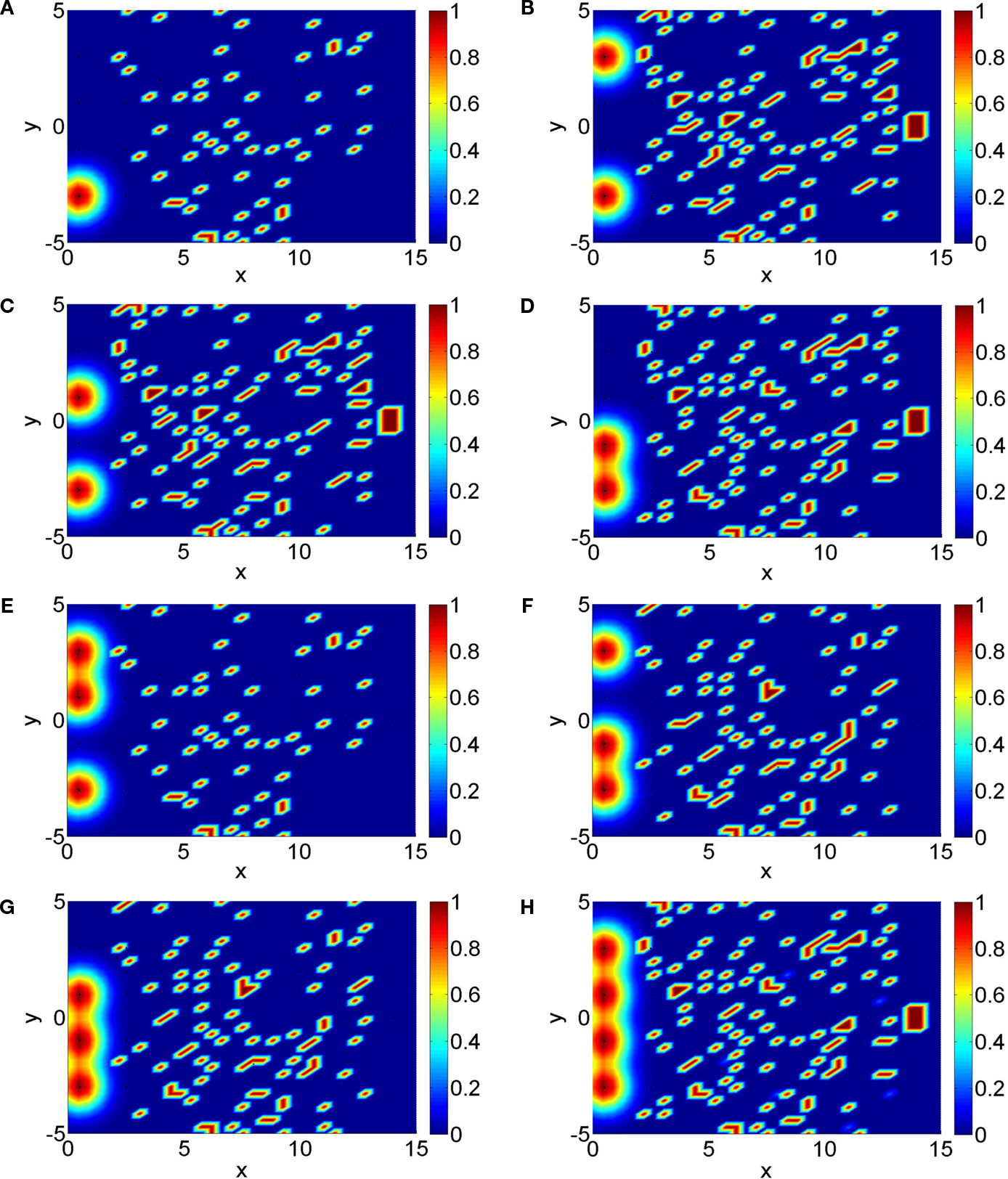
Figure 7. The images show the traces of neural pulses for the last binary digit of a gated binary addition logic (Eq. 35a–h) corresponding to the panels A–H via the basis transformation technique of Section “An Abstract View and Basis Transformations” in combination with the zero-dimensional embedding technique with purely analytical elements for the logical components of Section “Embedding 0D Logic into Neural Tissue”.
The time dynamics of these fields is illustrated in Figure 8
, where in a), b), c),…,h) we show snapshots of the fields at points tk in time for

with some appropriate constant k0 ∈ ℕ. It seems to show a random (“flickering”) dynamics of neural fields. But the logic which is implemented here is deterministic and according to the transformation (Eq. 52) equivalent to the pulse logic and zero-dimensional logic in the Figures 5
or 6
.
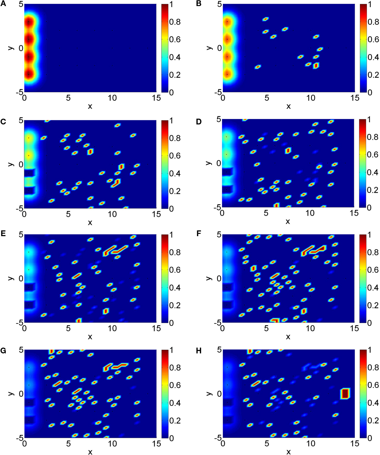
Figure 8. We illustrate the time dynamics of the distributed processing of 1 + 1 + 1 = 1 with gating pulse, displaying the neural field at eight time steps (Eq. 54) for k = 1 for panel A, k = 2 for panel B, k = 3 for panel C, k = 4 for panel D,k = 5 for panel E, k = 6 for panel F, k = 7 for panel G, k = 8 for panel H. The fields seem to show a random flickering due to the distributed nature of the basis activated basis elements. However, the binary logic is fully implemented in the distributed neural field dynamics and here leads to the desired excitation of the exit node as a result of the neural processing.
We have shown that neural field kernels can be constructed in a stable and computationally cheap way to carry out complex cognitive tasks using embedding techniques which map zero- or one-dimensional (computational or analytical) solutions into a higher-dimensional neural space.
Further, we have shown a variety of different implementations of complex logical tasks like binary addition with several input nodes. In particular, we have shown that we can achieve a stable and controllable
a) pulse-dynamics,
b) localized state dynamics and
c) distributed Hilbert space-based logical dynamics
in a neural field environment. This provides a basis for the further study of artificial or natural cognitive dynamics based on continuous connectionist structures.
For the one-dimensional embedding, we constructed local kernels for describing pulses that travel along directed continuous paths in the neural domain. This is essentially a continuous version of classical connectionist feed-forward architectures.
On the other hand, zero-dimensional embeddings combined with basis transformation techniques open a field for non-local neural field dynamics that has not been explored so far. In particular, the abstract Hilbert space representations could be useful for implementing even more complex tasks than logical computations in neural field models, for example dynamical language processing (Maye and Werning, 2007
; Werning and Maye, 2007
; beim Graben and Potthast, 2009
).
The oscillatory patterns observed in our simulations also highlight the functional significance of cortical oscillations in general (Basar, 1998
). Moreover, the chains of local random patches in the distributed dynamics that excite each other mutually can be regarded as operational cell assemblies as introduced by Wennekers (2006
, 2007)
. Hence the embedding of low-dimensional solutions of the neural inverse problem by means of Hilbert space basis transformations provide a promising way for the implementation of such processing architectures.
The authors declare that the research was conducted in the absence of any commercial or financial relationships that could be construed as a potential conflict of interest.
This research has been supported by an EPSRC Bridging the Gaps Award in the UK under grant number EP/F033036/1.