1
Bernstein Center for Computational Neuroscience, Freiburg, Germany
2
Computational Neuroscience, Faculty of Biology, Albert-Ludwig University, Freiburg, Germany
3
RIKEN Brain Science Institute, Wako City, Japan
4
Brain and Neural Systems Team, RIKEN Computational Science Research Program, Wako City, Japan
The integrate-and-fire neuron with exponential postsynaptic potentials is a frequently employed model to study neural networks. Simulations in discrete time still have highest performance at moderate numerical errors, which makes them first choice for long-term simulations of plastic networks. Here we extend the population density approach to investigate how the equilibrium and response properties of the leaky integrate-and-fire neuron are affected by time discretization. We present a novel analytical treatment of the boundary condition at threshold, taking both discretization of time and finite synaptic weights into account. We uncover an increased membrane potential density just below threshold as the decisive property that explains the deviations found between simulations and the classical diffusion approximation. Temporal discretization and finite synaptic weights both contribute to this effect. Our treatment improves the standard formula to calculate the neuron’s equilibrium firing rate. Direct solution of the Markov process describing the evolution of the membrane potential density confirms our analysis and yields a method to calculate the firing rate exactly. Knowing the shape of the membrane potential distribution near threshold enables us to devise the transient response properties of the neuron model to synaptic input. We find a pronounced non-linear fast response component that has not been described by the prevailing continuous time theory for Gaussian white noise input.
Reduced models of neurons and networks are useful tools for investigating prominent features of recurrent network dynamics, and serve as guides for biophysically more detailed models. The leaky integrate-and-fire neuron (Stein, 1965
) is such a widely used model, in which an incoming synaptic event causes an exponential postsynaptic potential of finite amplitude and a spike is emitted whenever the membrane potential reaches the firing threshold, followed by resetting the membrane potential to a fixed potential. This model is efficient to simulate and in certain regimes it is a good approximation of both more complicated neuron models (Izhikevich, 2004
) and of real neurons (Rauch et al., 2003
; La Camera et al., 2004
; Jovilet et al., 2008
). The analytic treatment of its dynamics has been performed in the diffusion limit (Siegert, 1951
; Ricciardi and Sacerdote, 1979
; Brunel, 2000
), where the input current is approximated as Gaussian white noise and the equilibrium solution is known exactly. Hohn and Burkitt (2001)
took into account finite synaptic weights to obtain the free membrane potential distribution and to solve the first passage time problem numerically. Richardson (2007
, 2008
) developed a numerical framework to calculate the equilibrium and response properties of linear and non-linear integrate-and-fire neurons. Here we extend the known analytic theory in two respects. Firstly, we go beyond a pure diffusion approximation and take into account finite postsynaptic potentials where their effect is most prominent: our new treatment still describes the probability density evolution on a length scale σ determined by the fluctuations in the input as a diffusion, but we take into account the discrete events near the absorbing boundary. With a different approach Sirovich et al. (2000) and Sirovich (2003)
calculated the equilibrium solution for finite sized excitatory incoming events. De Kamps (2003)
developed a stable numerical approach to solve the equilibrium and non-equilibrium population dynamics. Here we are interested in the case of excitatory and inhibitory inputs, as they occur in balanced neural networks (van Vreeswijk and Sompolinsky, 1996
; Brunel, 2000
). Secondly, unlike previous analytical treatments, we solve the problem in discrete time to incorporate the effect of the discretization on the equilibrium and response properties of the neuron. This is necessary to get a quantitative understanding of artifacts observed in simulation studies: in time-driven simulations, the state of the neuron is only updated in time steps of size h and the incoming synaptic impulses are accumulated over one such time step. However, modern time-driven simulators (Gewaltig and Diesmann, 2007
; Morrison et al., 2007
) are able to take into account exact spike timing and hence avoid discretization effects. These methods can be either slower or faster than traditional time-driven techniques depending on the required accuracy.
The threshold makes this model a non-linear input-output device, complicating a full analytic treatment of the dynamics. Linearization of the neuron around a given background input and treating deviations of the input from baseline as small perturbations is the usual solution. In this linear approximation, the response of the neuron is quantified by a response kernel. This approach enables the characterization of recurrent random networks by a phase diagram (Brunel and Hakim, 1999
; Brunel, 2000
), to explain stochastic resonance (Lindner and Schimansky-Geier, 2001
), to investigate feed-forward transmission of correlation (Tetzlaff et al., 2003
; De la Rocha et al., 2007
), and to disentangle the mutual interaction of spike-timing dependent synaptic learning rules and neural dynamics (Kempter et al., 1999
; Helias et al., 2008
; Morrison et al., 2008
). For large input transients (Goedeke and Diesmann, 2008
) recently devised an approximation of the spike density to investigate synchronization phenomena in synfire chains (Diesmann et al., 1999
).
For continuous time and in the diffusion limit, Brunel et al. (2001)
, Lindner and Schimansky-Geier (2001)
, and Fourcaud-Trocmé et al. (2003)
have calculated the linear response to periodic perturbations analytically and concluded, that the integrate-and-fire neuron acts as a low-pass filter. In contrast, we show that for finite postsynaptic potentials (and in discrete time) the neuron transmits changes in the input as fast as the time step h in a non-linear manner.
The structure of the paper is as follows: In Section “Density Equation for the Integrate-and-Fire Neuron” we state the model equations for the integrate-and-fire neuron and derive a Fokker–Planck equation describing the time evolution of the probability density function of the membrane potentials of a population of such neurons in discrete time. Section “Boundary Condition at the Threshold and Normalization” discusses the boundary conditions that apply to the probability density. Here we show that finite synaptic weights as well as the time step markedly influence the equilibrium properties (mean firing rate, stationary probability density). In Section “Accuracy and Limits of the Solution” we compare our result against simulations and a numerical solution to check the accuracy of our approximation. In Section “Response Properties” we investigate the response of the neuron to a brief perturbation of the membrane potential and we demonstrate an immediate non-linear response. Section “Discussion” puts our results into the context of computational neuroscience and discusses the applicability and limits of our theory.
We consider a leaky integrate-and-fire neuron (Lapicque, 1907
) that receives the input current I(t). The membrane potential is governed by the differential equation

with the membrane time constant τ and the membrane resistance R. Whenever the membrane potential reaches the voltage threshold Vθ, the neuron elicits a spike and the membrane potential is reset to Vr, where it is clamped for the absolute refractory time τr. The input current I(t) is brought about by excitatory and inhibitory point events from homogeneous Poisson processes with the rates νe and νi, respectively. Each synaptic input causes a δ-shaped (δ denotes the Dirac distribution) postsynaptic current, which leads to a jump in the membrane potential. The amplitude of an excitatory synaptic impulse is w, of an inhibitory impulse −gw,

We apply a diffusion equation approach (Brunel and Hakim, 1999
; Ricciardi et al., 1999
; Brunel, 2000
) to an ensemble of identical integrate-and-fire neurons characterized by Eqs. 1 and 2. The population is described by a probability density function P(V, t) of the membrane potential V. Unlike the above mentioned works, here we treat the problem in discrete time where the time t advances in time steps h. The case of continuous time can be obtained at any step in the limit h → 0. In discrete time, the probability density P(V, t) characterizes the system at regular time intervals. In this paper, we follow the convention that P(V, t), for t ∈ hℕ0, describes the density at the beginning of the time interval. We decompose the evolution of the membrane potential density into three steps: Decay, incoming events, and thresholding (Diesmann et al., 2001
). During the time interval (t, t + h), each neuron’s membrane potential Vi in the ensemble decays by a factor of e−h/τ and hence has the value Vie−h/τ at the end of the interval. This decay amounts to a shrinkage of the membrane potential density  as illustrated in Figure 1
A. We denote with
as illustrated in Figure 1
A. We denote with  the probability density function directly before the synaptic impulses in the current time interval are taken into account (Morrison and Diesmann, 2008
). At the end of the interval, all synaptic inputs that arrived within this interval are taken into account. They cause each individual membrane potential to jump by a discrete random number γ = wκe − wgκi, where κe and κi are the Poisson distributed random numbers of incoming excitatory and inhibitory events in the interval of length h, respectively. We denote with 𝒫(γ) the probability of the jump γ to occur. All membrane trajectories Vi that have crossed the threshold are reset to Vr, the corresponding neuron emits a spike and remains refractory for the time τr. This is equivalent to the probability flux at time t across the threshold being reinserted at the reset Vr at time t + τr. The time evolution is sketched in Figure 1
A. To solve for the equilibrium distribution, we have to find the distribution which is invariant to this cycle of three subsequent steps, so it must satisfy P(V, t + h) = P(V, t).
the probability density function directly before the synaptic impulses in the current time interval are taken into account (Morrison and Diesmann, 2008
). At the end of the interval, all synaptic inputs that arrived within this interval are taken into account. They cause each individual membrane potential to jump by a discrete random number γ = wκe − wgκi, where κe and κi are the Poisson distributed random numbers of incoming excitatory and inhibitory events in the interval of length h, respectively. We denote with 𝒫(γ) the probability of the jump γ to occur. All membrane trajectories Vi that have crossed the threshold are reset to Vr, the corresponding neuron emits a spike and remains refractory for the time τr. This is equivalent to the probability flux at time t across the threshold being reinserted at the reset Vr at time t + τr. The time evolution is sketched in Figure 1
A. To solve for the equilibrium distribution, we have to find the distribution which is invariant to this cycle of three subsequent steps, so it must satisfy P(V, t + h) = P(V, t).
as illustrated in Figure 1
A. We denote with the probability density function directly before the synaptic impulses in the current time interval are taken into account (Morrison and Diesmann, 2008
). At the end of the interval, all synaptic inputs that arrived within this interval are taken into account. They cause each individual membrane potential to jump by a discrete random number γ = wκe − wgκi, where κe and κi are the Poisson distributed random numbers of incoming excitatory and inhibitory events in the interval of length h, respectively. We denote with 𝒫(γ) the probability of the jump γ to occur. All membrane trajectories Vi that have crossed the threshold are reset to Vr, the corresponding neuron emits a spike and remains refractory for the time τr. This is equivalent to the probability flux at time t across the threshold being reinserted at the reset Vr at time t + τr. The time evolution is sketched in Figure 1
A. To solve for the equilibrium distribution, we have to find the distribution which is invariant to this cycle of three subsequent steps, so it must satisfy P(V, t + h) = P(V, t).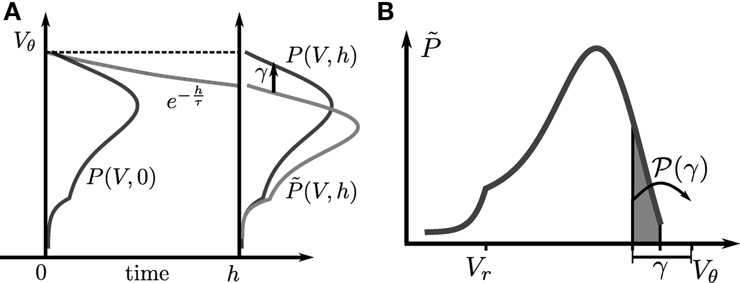
Figure 1. (A) Evolution of the membrane potential distribution between two adjacent time steps t = 0 and t = h. At the beginning of the interval, the distribution is P(V, 0). Each individual membrane potential in the ensemble then decays exponentially with the membrane time constant τ resulting in a contracted distribution  At the end of the interval the synaptic inputs are taken into account which cause a redistribution of the membrane potentials. All membrane trajectories exceeding the threshold Vθ elicit a spike in the interval and the corresponding Vi is reset to Vr. In equilibrium, the distribution after one such cycle is identical to the initial distribution P(V, h) = P(V, 0) again. (B) Boundary condition at the threshold. The neuron receives synaptic inputs during a time step of length h. Their summed effect causes the membrane potential to perform a jump of random size γ with distribution 𝒫(γ). The figure shows one particular realization of γ. For positive γ (as indicated) the shaded area
  of the distribution is shifted above threshold in this time step and contributes to the firing rate (probability flux over the threshold). Each such contribution is weighted by the probability 𝒫(γ) for the jump γ to occur.
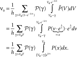
At the end of the interval the synaptic inputs are taken into account which cause a redistribution of the membrane potentials. All membrane trajectories exceeding the threshold Vθ elicit a spike in the interval and the corresponding Vi is reset to Vr. In equilibrium, the distribution after one such cycle is identical to the initial distribution P(V, h) = P(V, 0) again. (B) Boundary condition at the threshold. The neuron receives synaptic inputs during a time step of length h. Their summed effect causes the membrane potential to perform a jump of random size γ with distribution 𝒫(γ). The figure shows one particular realization of γ. For positive γ (as indicated) the shaded area of the distribution is shifted above threshold in this time step and contributes to the firing rate (probability flux over the threshold). Each such contribution is weighted by the probability 𝒫(γ) for the jump γ to occur.To formalize this approach, we follow Ricciardi et al. (1999) and assume that the main contributions to the time evolution of the membrane potential distribution can be described by an infinitesimal drift and a diffusion term. This is true as long as synaptic amplitudes are small (w ≪ Vθ − Vr). However, in the region near the threshold Vθ we treat the finite synaptic weights separately giving rise to the boundary condition described in Section “Boundary Condition at the Threshold and Normalization”. The complete derivation of the Fokker–Planck equation for discrete time can be found in Section “Derivation of the Fokker–Planck Equation” in Appendix. We find it convenient to introduce the dimensionless voltage y and the dimensionless probability density Q defined as
where we introduced the mean μ: = wτ (νe − gνi) and variance σ2 := τw2(νe + g2νi) of the equivalent Gaussian white noise matching the first and second moment of the incoming synaptic events as well as the neuron’s equilibrium firing rate ν0. Subsequently we use the shorthands yθ = y(Vθ) and yr = y(Vr). For the equilibrium case the probability flux operator S can be expressed in terms of the dimensionless voltage y, acting on Q as

We drop the time dependence of both P and Q in what follows. The density in equilibrium has to fulfill the stationary Fokker–Planck equation (Eq. 22) which is equivalent to a piecewise constant probability flux
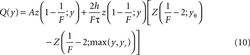
because the neuron spikes with its mean firing rate ν0, which equals the probability flux between reset and threshold. For yr ≤ y ≤ yθ Eq. 5 is a linear ordinary differential equation of first order so the general solution is a sum of a particular (Qp) and the homogeneous solution (Qh)

The constant A has to be determined from the boundary condition (see Section “Boundary Condition at the Threshold and Normalization”). The homogeneous solution satisfies SQh(y) = 0 so it has the form (see Section “General Solution of the Flux Differential Equation” in Appendix).
with

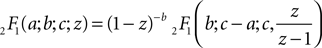
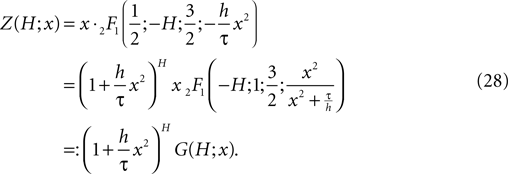
Here 2F1(a, b, c ; z) denotes the Gauss hypergeometric series (Abramowitz and Stegun, 1974
). We obtain the particular solution of Eq. 5 by variation of constants, which yields
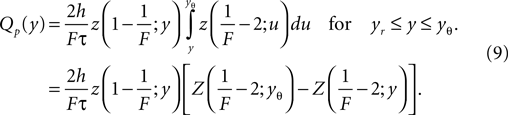
In the second line we used Z(H; y) as a shorthand for the integral of z(H; y), as defined in Eq. 27. We choose the upper bound yθ of the integral such that Qp(yθ) = 0. In order for the complete solution to be continuous at yr, the general solution of Eq. 5 reads
To determine the constant A appearing in Eq. 10, we need to consider the boundary condition at the threshold. Figure 1
B sketches the main idea: The probability flux over the threshold during one time step h is caused by those membrane potential trajectories which are carried over the threshold by the stochastic input within this time step. With γ denoting the discrete jump of the membrane potential due to the sum of excitatory and inhibitory inputs received in the current time step h, the probability mass crossing the threshold is  Here
Here  is the probability density observed prior to spike arrival at the end of the time step (as described in Section “Density Equation for the Integrate-and-Fire Neuron”). The membrane potential jump γ is caused by the synaptic inputs and hence is a random variable with a probability 𝒫(γ) (Eq. 29, Section “Boundary Condition at the Threshold” in Appendix). A threshold in a clock driven simulation can therefore alternatively be interpreted as a soft absorbing boundary: Within a simulation time step it may temporarily be crossed without producing a spike, as long as the net sum of excitatory and inhibitory synaptic events during the time step does not drive the membrane voltage above threshold.
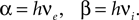
Here is the probability density observed prior to spike arrival at the end of the time step (as described in Section “Density Equation for the Integrate-and-Fire Neuron”). The membrane potential jump γ is caused by the synaptic inputs and hence is a random variable with a probability 𝒫(γ) (Eq. 29, Section “Boundary Condition at the Threshold” in Appendix). A threshold in a clock driven simulation can therefore alternatively be interpreted as a soft absorbing boundary: Within a simulation time step it may temporarily be crossed without producing a spike, as long as the net sum of excitatory and inhibitory synaptic events during the time step does not drive the membrane voltage above threshold.We express the membrane potential density  prior to spike arrival by the probability density at the beginning of the time step P as
  Our main assumption is that the shape of the density is to a good approximation described by the general solution (Eq. 10) of the corresponding diffusion process and hence varies on a length scale σ determined by the fluctuations in the input. Note that
  for V ≥ Vθe−h/τ due to the decay within one time bin (compare Figure 1
A). So the membrane potential jump γ must be positive and it must satisfy γ > Vθ − Vθe−h/τ = VθF in order to contribute to the flux (see Figure 1
B). The total flux over the threshold equals the firing rate ν0 of the neuron. So we obtain the condition
for V ≥ Vθe−h/τ due to the decay within one time bin (compare Figure 1
A). So the membrane potential jump γ must be positive and it must satisfy γ > Vθ − Vθe−h/τ = VθF in order to contribute to the flux (see Figure 1
B). The total flux over the threshold equals the firing rate ν0 of the neuron. So we obtain the condition
prior to spike arrival by the probability density at the beginning of the time step P as Our main assumption is that the shape of the density is to a good approximation described by the general solution (Eq. 10) of the corresponding diffusion process and hence varies on a length scale σ determined by the fluctuations in the input. Note that for V ≥ Vθe−h/τ due to the decay within one time bin (compare Figure 1
A). So the membrane potential jump γ must be positive and it must satisfy γ > Vθ − Vθe−h/τ = VθF in order to contribute to the flux (see Figure 1
B). The total flux over the threshold equals the firing rate ν0 of the neuron. So we obtain the condition
A similar condition appears in the case of excitatory synaptic events in continuous time (Sirovich, 2003
). We express P(V) by Q(y) using the general solution (Eq. 10) and solve for the constant A, which yields
with
For the details of the derivation see Section “Boundary Condition at the Threshold” in Appendix, where we also give an expression to evaluate the integrals using a Taylor expansion of Q(y) at the threshold utilizing Eq. 35
with
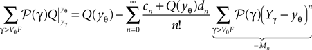
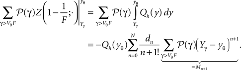
Here, Mn is the n-th rectified moment of the distribution 𝒫 of the membrane potential jumps due to synaptic input and cn is the n-th derivative evaluated at the threshold  It is obtained from the recurrence relation (Eq. 33) derived in Section “Boundary Condition at the Threshold” in Appendix. Note that this boundary condition fixes the value of the density at the threshold Q(yθ) = AQh(yθ), so we have expressed the non-local boundary condition (Eq. 11) (containing integrals of P) by a Dirichlet boundary condition at threshold yθ (Eq. 13).
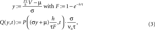
It is obtained from the recurrence relation (Eq. 33) derived in Section “Boundary Condition at the Threshold” in Appendix. Note that this boundary condition fixes the value of the density at the threshold Q(yθ) = AQh(yθ), so we have expressed the non-local boundary condition (Eq. 11) (containing integrals of P) by a Dirichlet boundary condition at threshold yθ (Eq. 13).In the diffusion limit the probability density vanishes at the threshold P(Vθ) = 0. This is mandatory because the infinitely high rate of incoming excitatory events would instantly deplete the states just below threshold. On the other hand, if the density did not vanish at the threshold this would imply an infinitely high firing rate of the neuron itself. Here in contrast, taking finite synaptic weights and finite incoming synaptic input rates into account, a value  at the threshold is compatible with the boundary condition, as can be seen from Figure 2
B. In addition, the time discretization even promotes this effect which can readily be understood: The density decays during a time step, so the highest voltage occupied by a neuron is Vθe−h/τ at the end of the time step, resulting in a gap of the density of size Vθ(1 − e−h/τ) just below threshold. The value of the membrane potential density at the threshold is the outcome of an equilibrium between the diffusive influx from left and the outflux over the boundary to the right. If the gap reduces the outflux, the density P(Vθ) will settle at an even higher value. Figure 6
A visualizes the effect for different temporal resolutions.
at the threshold is compatible with the boundary condition, as can be seen from Figure 2
B. In addition, the time discretization even promotes this effect which can readily be understood: The density decays during a time step, so the highest voltage occupied by a neuron is Vθe−h/τ at the end of the time step, resulting in a gap of the density of size Vθ(1 − e−h/τ) just below threshold. The value of the membrane potential density at the threshold is the outcome of an equilibrium between the diffusive influx from left and the outflux over the boundary to the right. If the gap reduces the outflux, the density P(Vθ) will settle at an even higher value. Figure 6
A visualizes the effect for different temporal resolutions.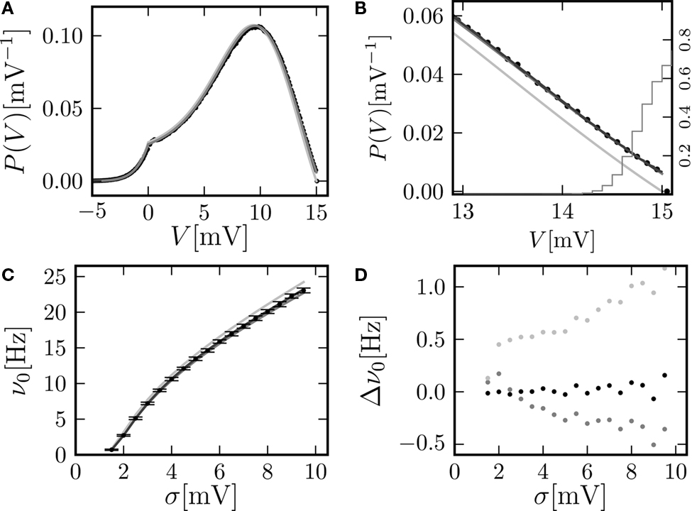
Figure 2. (A) Membrane potential distribution in equilibrium (Eq. 10) (gray), theory in diffusion limit neglecting finite synaptic weights and discrete time (light gray) from Brunel (2000) and direct simulation (black dots) binned to ΔV = 0.1 mV. Neuron parameters: Neuron parameters: τ = 20 ms, Vθ = 15.0 mV, Vr = 0, w = 0.1 mV, g = 4, τr = 1 ms. Incoming synaptic rate νe = 29800 Hz, νi = 5950 Hz (corresponding to μ = 12.0 mV and σ = 5.0 mV). Time discretization h = 0.1 ms. (B) Zoom in of (A). In addition the numerical solution of the Markov process according to Section “Numerical Solution of the Equilibrium distribution” in Appendix is displayed (dark gray; discretization ΔV = 0.01 mV). The probability of the membrane potential jumping across threshold in a time step h is given as light gray steps. (C) Equilibrium firing rate as a function of the fluctuations σ in the input from theory (Eq. 14) (gray), direct simulation (black error bars), theory neglecting finite weights and discrete time (light gray) and numeric solution of the Markov process (Eq. 37) (dark gray). Same parameters as in A, but νe, νi chosen to realize mean input μ = 5.0 and the fluctuation σ as given by the abscissa. (D) Deviation of analytic firing rate (Eq. 14) (gray), of the numerically obtained rate according to Section “Numerical Solution of the Equilibrium distribution” in Appendix (black), and of the rate in diffusion limit from Brunel (2000)
(light gray) with respect to the directly simulated rate.
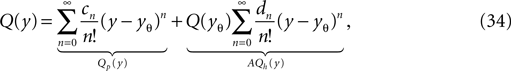
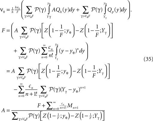
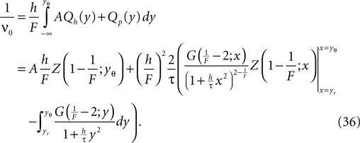
The calculation of the normalization condition of the probability density function (see Section “Normalization” in Appendix) determines the equilibrium firing rate ν0 of the neuron as
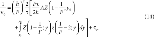
In particular for small σ it is necessary to transform the integrand in the second term to a numerically well-behaved function (Eq. 36) as given in Section “Normalization” in Appendix.
Knowing the normalization constant, we can use Eq. 10 together with Eq. 3 to compare the probability density P(V) to direct simulation (using NEST; Gewaltig and Diesmann, 2007
) and to the existing theory (Ricciardi and Sacerdote, 1979
; Brunel, 2000
) in the diffusion limit, see Figure 2
A. Although we chose synaptic weights w = 0.1 mV ≪ Vθ − Vr = 15.0 mV and small simulation time steps h = 0.1 ms, especially at the threshold there is a pronounced deviation of the simulated density from the one obtained in the diffusion limit. Figure 2
C graphs the dependence of the neuron’s Firing rate on the strength of fluctuations σ in the input.. The pure diffusion approximation exhibits a consistent overestimation of the simulated rate, whereas our solution (Eq. 14) shows only a slight underestimation, as can be seen in Figure 2
D in more detail.
To check the accuracy of our theory, we compare it to a numerically obtained solution for the equilibrium distribution and firing rate. To this end we model the membrane potential as a Markov process the state of which is completely determined by the membrane potential distribution P(V, t) which undergoes transitions between adjacent time steps. These transitions are composed of the sequence of decay (D), voltage jumps due to synaptic input (J) and the thresholding operation (T). We discretize the voltage axis and determine the composed transition matrix TJD between discrete voltage bins. Due to the Perron–Frobenius theorem (MacCluer, 2000
), the column-stochastic transition matrix [satisfying Σj(TJD)ij = 1 ∀i] has an eigenvalue 1 that corresponds to the equilibrium state. We determine the corresponding eigenvector numerically which yields the equilibrium distribution and allows to calculate the firing rate. For details see Section “Numerical Solution of the Equilibrium Distribution” in Appendix.
Figure 3
A shows the probability density obtained by the three different methods: Direct simulation, numerical solution of the Markov system, and theory (Eq. 10). The agreement of all three variables in the relevant range below the threshold is excellent. However, the equilibrium firing rate shows a deviation of up to 0.5 Hz (Figure 2
D). Compared to the frequently applied pure diffusion approximation, this is an improvement by a factor of about 2. The numerical solution agrees within the limits of the rate estimation. The limited precision of the analytic treatment is explained by the detailed shape of the probability density just below threshold (Figure 3
A): The numerically determined density exhibits a modulation on a scale much smaller than the scale σ of the analytic solution. It is determined by a combination of temporal discretization and non-vanishing synaptic weights. If the synaptic weights are sufficiently large (in Figure 3
A at w = 0.15, 0.25 mV) the effect of the time discretization becomes apparent. The observed modulation has a periodicity of  equal to the decay of the membrane voltage near threshold within one time step. The zoom-in shown in Figure 3
C confirms this numeric value. However, if the synaptic weights are sufficiently small (in Figure 3
A at w = 0.05 mV) the modulation is reduced, because the synaptic jumps then mix adjacent states in a similar voltage range.
equal to the decay of the membrane voltage near threshold within one time step. The zoom-in shown in Figure 3
C confirms this numeric value. However, if the synaptic weights are sufficiently small (in Figure 3
A at w = 0.05 mV) the modulation is reduced, because the synaptic jumps then mix adjacent states in a similar voltage range.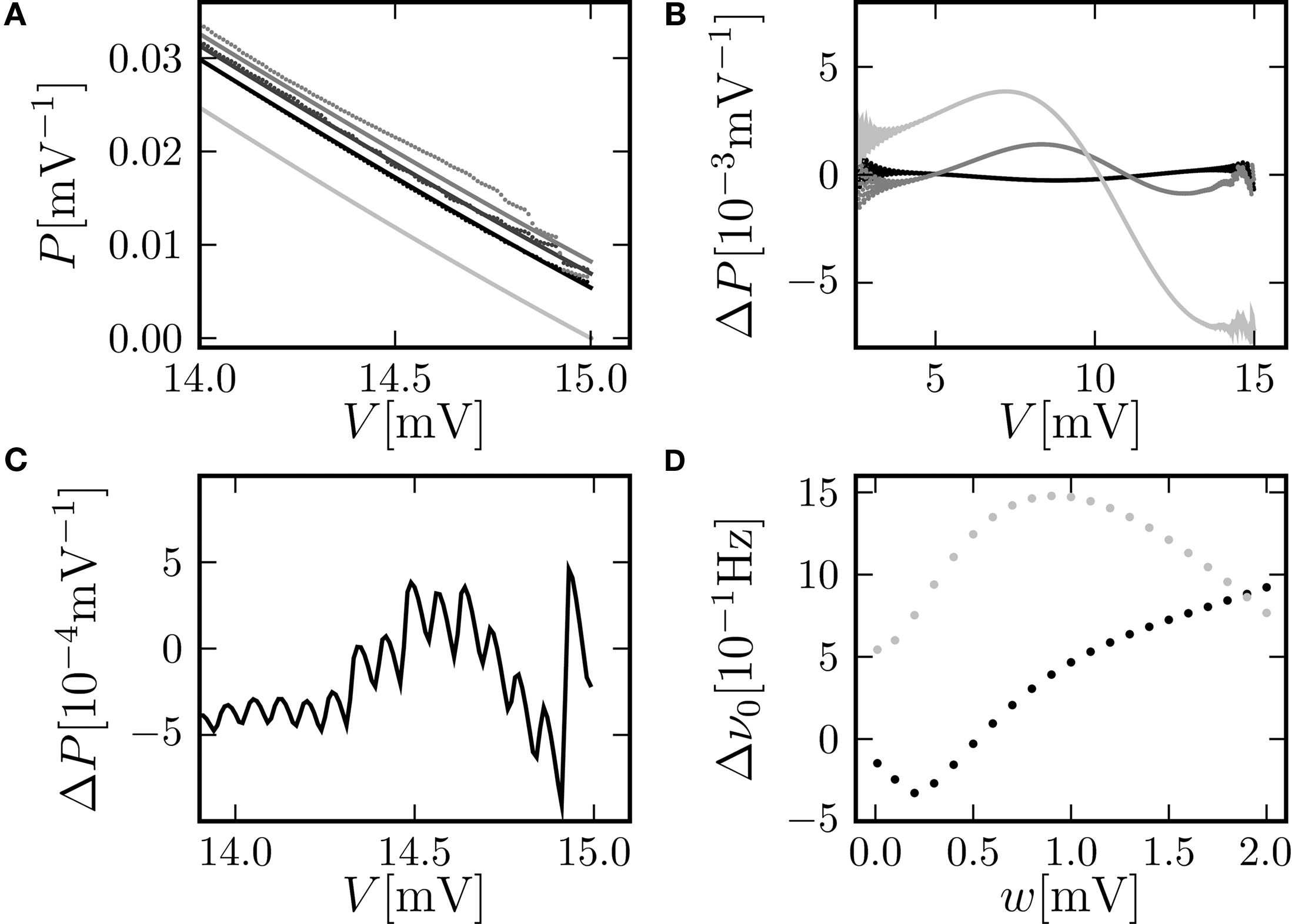
Figure 3. (A) Membrane potential distribution near threshold for fixed μ = 12. 0 and σ = 5.0 but different synaptic weights (black: w = 0.05 mV, dark gray: w = 0.15 mV, gray: w = 0.25 mV). Numerical solution of the Markov process according to Section “Numerical Solution of the Equilibrium distribution” in Appendix (dotted lines, discretization ΔV = 0.01 mV), analytic solution (Eq. 10) (solid line) and theory in diffusion limit neglecting finite synaptic weights and discrete time (light gray) from Brunel (2000)
. (B) Deviation ΔP = Pana = Pnum of the analytic membrane potential distribution (Eq. 10) from the numerically obtained distribution from Section “Numerical Solution of the Equilibrium distribution” in Appendix (black: w = 0.15 mV; g = 1.0, gray: w = 0.15, g = 4). Discrepancy between the diffusion approximation (Brunel, 2000
) and the numerically obtained solution described in Section “Numerical Solution of the Equilibrium distribution” in Appendix (light gray: w = 0.15 mV, g = 4). (C) Zoom in of (B) for w = 0.15 mV, g = 4. (D) Error of the analytic firing rate (Eq. 14) (black) and of the pure diffusion approximation (light gray) compared to the numerically obtained rate from Section “Numerical Solution of the Equilibrium distribution” in Appendix for different synaptic amplitudes w. Further parameters as in Figure 2
A.
Figure 3
B shows the deviation of the analytical approximation for the membrane potential distribution from the close to exact numerical solution of the Markov system. The new boundary condition (Eq. 13) improves the agreement close to threshold compared to the pure diffusion approximation. However, even far away from threshold and varying on a voltage scale σ there is still a deviation, which is qualitatively proportional to the derivative of the density. This amounts to a shift along the voltage axis of the analytical and the numerical result. This deviation largely vanishes for a more symmetric jump distribution (g = 1, black graph in Figure 3
B). This indicates the truncation of the Kramers–Moyal expansion after the second term to be the reason, because it is equivalent to neglecting all cumulants of the jump distribution beyond order 2, and in particular neglecting its skewness in the unbalanced case (g ≠ 1).
Figure 3
D displays the deviation of the analytically derived firing rate from the numerical result for different synaptic amplitudes w. For a large range of synaptic weights, the new approximation is better than the pure diffusion approximation. Only near the maximum possible weight 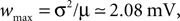 defined by the condition of a positive inhibitory rate, the new approximation becomes slightly worse than the pure diffusion approximation. However, in this range any diffusion approximation is expected to fail, because already a small number of synaptic events (. 8) drives the neuron from reset to threshold.
defined by the condition of a positive inhibitory rate, the new approximation becomes slightly worse than the pure diffusion approximation. However, in this range any diffusion approximation is expected to fail, because already a small number of synaptic events (. 8) drives the neuron from reset to threshold.We now explore further consequences of the non-vanishing membrane potential density just below threshold. We suspect the response properties of the neuron to be affected, because an increased density below threshold means that there are more neurons brought to fire by a small positive deflection of the membrane potential. Previous analytical work (Brunel et al., 2001
) showed that synaptic filtering increases the density below threshold and hence leads to an immediate response of the neuron. In this section we demonstrate a comparable effect due to finite synaptic weights and time discretization.
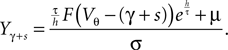
The response of a neuron to an impulse-like additional input of amplitude s is of particular interest: It allows to calculate the correlation between the incoming spike train and the spiking activity produced by the neuron itself. Up to linear approximation, the impulse response uniquely determines the system. Here, we present two characteristic features of this response with respect to an impulse-like perturbation of the membrane potential: First, we calculate its integral over time nr (Eq. 15). This can be understood as the total number of additional (s > 0) or suppressed (s < 0) action potentials of the neuron due to the perturbation. Secondly, we look at the instantaneous firing rate directly after the perturbation occurred. This is an interesting quantity, because an immediate response to an input enables the neuron to transmit information from the input to the output with arbitrary speed.
A δ-impulse, which can be understood as the limit of a very short but very strong current injection with integral 1, produces a deterministic change of the membrane potential by u(t) within a given time step. Eq. 23 shows that this perturbation can be considered as a time dependent mean input 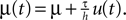 If the neuron was in equilibrium before, without loss of generality, we can assume this perturbation to take place in the time step (0,h). Within this interval the membrane potential changes deterministically by u(t): = sδt,0, where s is the amplitude of the jump the membrane potential performs. We understand t as the discrete time advancing in steps of h and δi,j = 1 if i = j and 0 otherwise (Kronecker symbol). In the continuous limit h → 0, this would be equivalent to an impulse like current injection RI(t) = τsδ(t). First, we are interested in the integral response nr of the neuron’s firing rate
If the neuron was in equilibrium before, without loss of generality, we can assume this perturbation to take place in the time step (0,h). Within this interval the membrane potential changes deterministically by u(t): = sδt,0, where s is the amplitude of the jump the membrane potential performs. We understand t as the discrete time advancing in steps of h and δi,j = 1 if i = j and 0 otherwise (Kronecker symbol). In the continuous limit h → 0, this would be equivalent to an impulse like current injection RI(t) = τsδ(t). First, we are interested in the integral response nr of the neuron’s firing rate
also called “DC-susceptibility”. In linear approximation (in linear response theory), the deviation of the neuron’s firing rate from its equilibrium rate is called “impulse response” of the firing rate. From the theory of linear systems we know that the integral of the impulse response equals the step response of the system. Hence Eq. 15 can be written up to the linear terms as

To calculate  , where
  is given by Eq. 14, we also need to take into account the dependence of A on μ. The straightforward but lengthy calculation can be found in Section “Response of Firing Rate to Impulse like Perturbation of Mean Input” in Appendix, which leads to
, where is given by Eq. 14, we also need to take into account the dependence of A on μ. The straightforward but lengthy calculation can be found in Section “Response of Firing Rate to Impulse like Perturbation of Mean Input” in Appendix, which leads to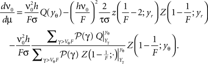
There, we also derive a recurrence relation for the derivatives of Q to evaluate the sums appearing in the last term. Eq. 16 shows the integral response for a positive and a negative perturbation to be symmetric to linear approximation in a whole range of firing rates (the range of σ results in the firing rates of Figure 2
C). Especially at low σ, the linear approximation exhibits a pronounced deviation from direct simulation results. At fixed σ = 5.0 mV, Figure 4
C shows the very good agreement of this linear approximation for sufficiently small perturbations and also slight deviations, as expected, at larger positive values. These deviations are discussed below.
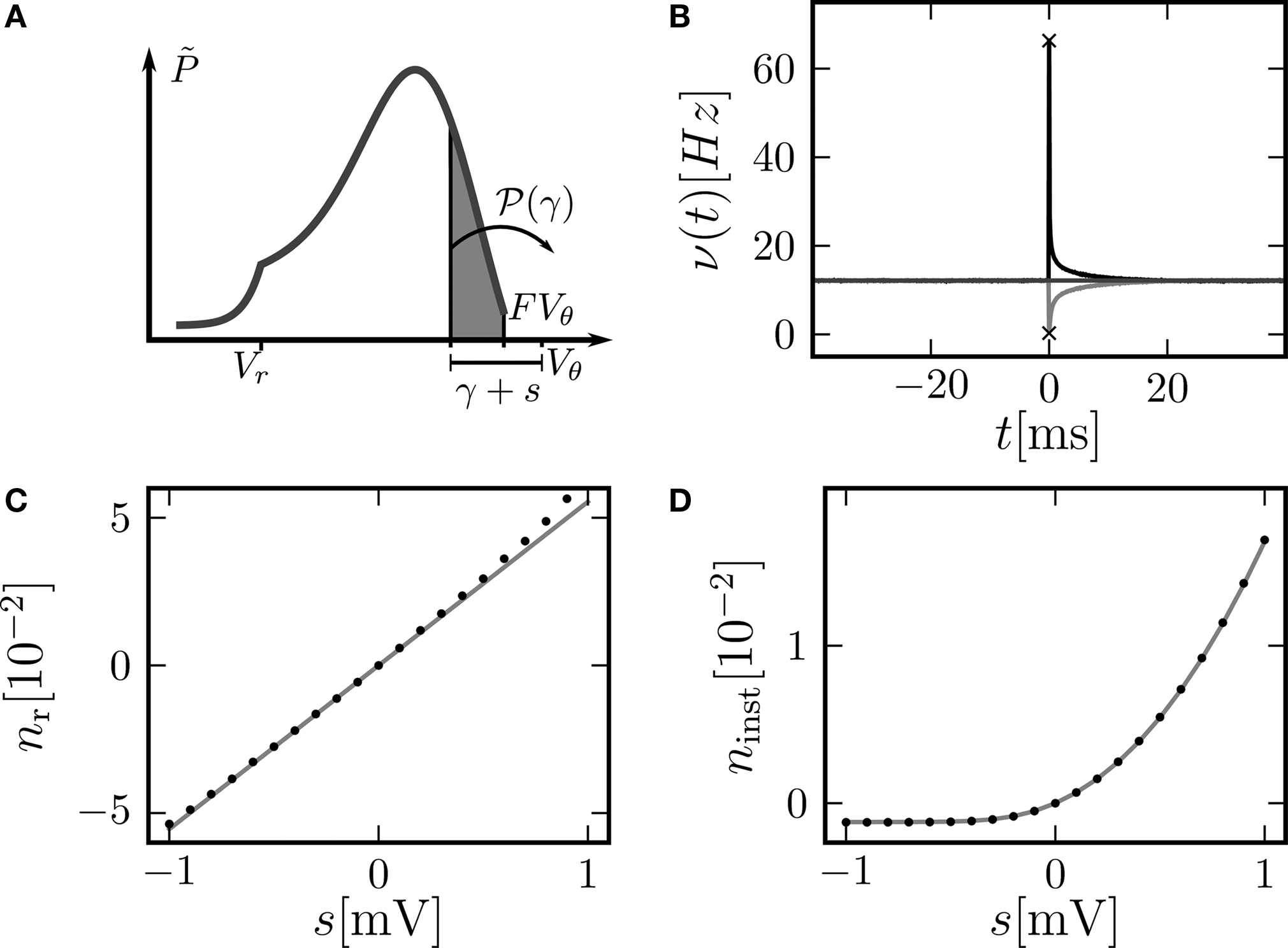
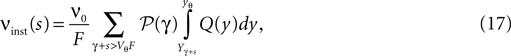
Figure 4. (A) Illustration of the instantaneous firing rate due to a perturbation of size s: During the time bin h, synaptic inputs cause a jump γ of the membrane potential in addition to the perturbation s. The probability mass (shaded area) is shifted above threshold with probability 𝒫(γ) and produces the response of the neuron. Due to the shape of the probability density near the threshold, this area has a linearly [proportional to sP(Vθ), area of the rectangular base] and a quadratically increasing contribution [proportional to  , area of the triangle] in s. (B) Firing rate as function of time after a perturbation of size s = 0.5 mV (upper trace) and of size s = −0.5 mV (lower trace) in the time bin [0, h). The black crosses denote the analytic peak response given by Eq. 17 for both cases. Solid curves from direct simulation of the response. Parameters as in Figure 2
, but incoming synaptic rates νe = 29600 Hz, νi = 5962.5 Hz (corresponding to μ = 11.5 mV and σ = 5.0 mV). (C) Integral response (Eq. 15) (gray) depending on the strength of the perturbation, direct simulation (black dots). (D) Instantaneous response depending on the strength of the perturbation s. Theory using Eq. 17 (gray) and direct simulation (black). Other parameters in (C,D) as in (B).
, area of the triangle] in s. (B) Firing rate as function of time after a perturbation of size s = 0.5 mV (upper trace) and of size s = −0.5 mV (lower trace) in the time bin [0, h). The black crosses denote the analytic peak response given by Eq. 17 for both cases. Solid curves from direct simulation of the response. Parameters as in Figure 2
, but incoming synaptic rates νe = 29600 Hz, νi = 5962.5 Hz (corresponding to μ = 11.5 mV and σ = 5.0 mV). (C) Integral response (Eq. 15) (gray) depending on the strength of the perturbation, direct simulation (black dots). (D) Instantaneous response depending on the strength of the perturbation s. Theory using Eq. 17 (gray) and direct simulation (black). Other parameters in (C,D) as in (B).Another quantity of interest is the instantaneous response of the neuron to the impulse-like perturbation. In the framework of discrete time, the fastest response possible is the emission of a spike in the same time step as the neuron receives the perturbation (this preserves causality; Morrison and Diesmann, 2008
). We call this the “instantaneous response”. To quantify the response we follow similar arguments as in Section “Boundary Condition at the Threshold and Normalization” and determine the probability mass crossing the threshold within the time step when the perturbation s occurred. Just prior to the perturbation we assume the neuron to be in equilibrium, hence its membrane potential distribution is given by Q(y). We have to take into account the additional deterministic change of membrane potential u(t): = sδt,0 caused by the perturbation in the condition for the firing rate (Eq. 11). The instantaneous rate in the time bin of the perturbation is then caused by the deterministic change s superimposed with all stochastically arriving synaptic impulses whose summed effect on the membrane potential is a jump γ
with
As in Section “Boundary Condition at the Threshold” in Appendix, we evaluate the integral using the series expansion of Q at the threshold employing Eqs. 34 and 35. We obtain for the instantaneous rate
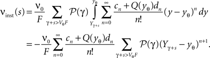
The sequences cn and dn are derived in Section “Boundary Condition at the Threshold” in Appendix, Eq. 33. For small perturbations of the order of a synaptic weight, the series can be truncated at low n. Throughout this paper we use n = 3. From this expression we see, that the lowest order terms of the response are linear and quadratic in the size of the perturbation s. The linear term (n = 0) is proportional to Q(yθ), the quadratic term to −Q′(yθ). Geometrically this can be understood from Figure 4
A: the shaded area is proportional to the instantaneous firing rate and increases to good approximation with the linear term sP(Vθ) (area of the rectangular base) and the quadratic term  (area of the triangle).
(area of the triangle).This non-linearity can readily be observed. Figure 4
B shows a typical rate transient for a positive perturbation and a negative perturbation of equal magnitude. The resulting immediate rate deflection for the positive perturbation is much more pronounced, while the following tail of the response is more symmetric in both cases. To compare the instantaneous response to the integral response nr we look at the number of spikes ninst produced (s > 0) or suppressed (s < 0) in comparison with the base rate in the time step of perturbation

Figure 4
D shows the dependence of this instantaneous response ninst on the strength of the perturbation. In contrast to the integral response, even at small perturbations of the order of a single synaptic weight the instantaneous response is strongly non-linear and has a rectifying effect, reflecting the fact that negative perturbations have a much weaker effect than positive ones. Theory and direct simulation fit to high accuracy for a large range of different levels of fluctuation σ, as shown in Figure 5
B. There is an optimal level of fluctuations around σ ≃ 3 mV to foster the direct response to a positive perturbation which can be interpreted as stochastic resonance. For periodic input signals stochastic resonance has been described before (Lindner and Schimansky-Geier, 2001
) and for slow transient inputs an adiabatic approximation can explain this aperiodic stochastic resonance (Collins et al., 1996
). Figures 5
C,D reveal the reason for the response to fast transients to depend on the strength of noise. The probability density just below threshold assumes a maximum for an intermediate magnitude of fluctuations (middle gray curve, σ = 3 mV), resulting in a maximum of probability to be shifted across threshold by a small perturbation. The density below threshold is determined by two competing effects: At low levels of noise, increasing the fluctuations spreads out the density, pushing it closer to the threshold and therefore promoting the response. Further increasing the fluctuations, the rectifying nature of the absorbing boundary gains importance, since a positive fluctuation easily leads to a threshold crossing and absorption of the state in contrast to negative fluctuations. Effectively, this results in a net drift to lower voltages, decreasing the density near threshold and therefore the response. The contribution of the instantaneous response to the integral response is not captured by the linear theory (Eq. 16) by definition. This explains the positive deviation between simulation and the linear expectation observed in Figure 5
A for the positive perturbation at low σ and the deviation in Figure 4
C at large positive s. It shows the limits of validity for the linear perturbation theory for large perturbations (≃1 mV).
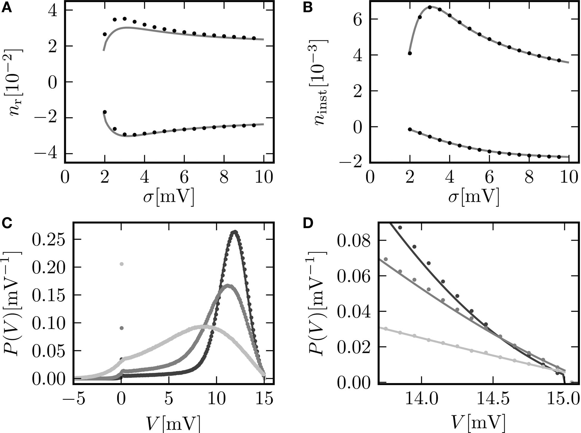
Figure 5. (A) Integral response nr (Eq. 15) for perturbation s = 0.5 mV (upper graph) and s = −0.5 mV (lower graph) as a function of the fluctuations σ of synaptic input. Theoretical prediction (Eq. 16) (gray) and direct simulation (black dots). (B) Instantaneous response ninst (Eq. 18) to a perturbation s = 0.5 mV (top graph) and to a perturbation s = −0.5 mV (bottom graph). Analytic result using Eq. 17 (gray) and direct simulation (black dots). (C,D) P.d.f. of the membrane potential for σ∈{2, 3, 6} mV shown in dark gray, gray and light gray, respectively. Other parameters as in Figure 2
C.
The time step of the simulation has an effect on the boundary condition at the firing threshold, as outlined in Section “Boundary Condition at the Threshold and Normalization”. Figure 6
A shows the detailed shape of the membrane potential distribution just below threshold: For coarser time discretization the value at the boundary increases. Consequently, the instantaneous response of the neuron to a perturbation within the same time step increases as well (not shown). For a fair comparison, however, we integrated the response over the same time interval for all time resolutions. This is shown in Figure 6
B. For positive perturbations a coarser time discretization increases the response only marginally. The threshold-nonlinear behavior observed for perturbations around s = 0, however, is linearized by larger time steps, as can be seen by comparing Figure 6
B (for h = 0.5 ms) to Figure 4
D (for h = 0.1 ms). The reason is the linear increase of the variance of the accumulated synaptic events in proportion to the time step h, diminishing the relative contribution of the perturbation and therefore weakening the non-linearity around s = 0.
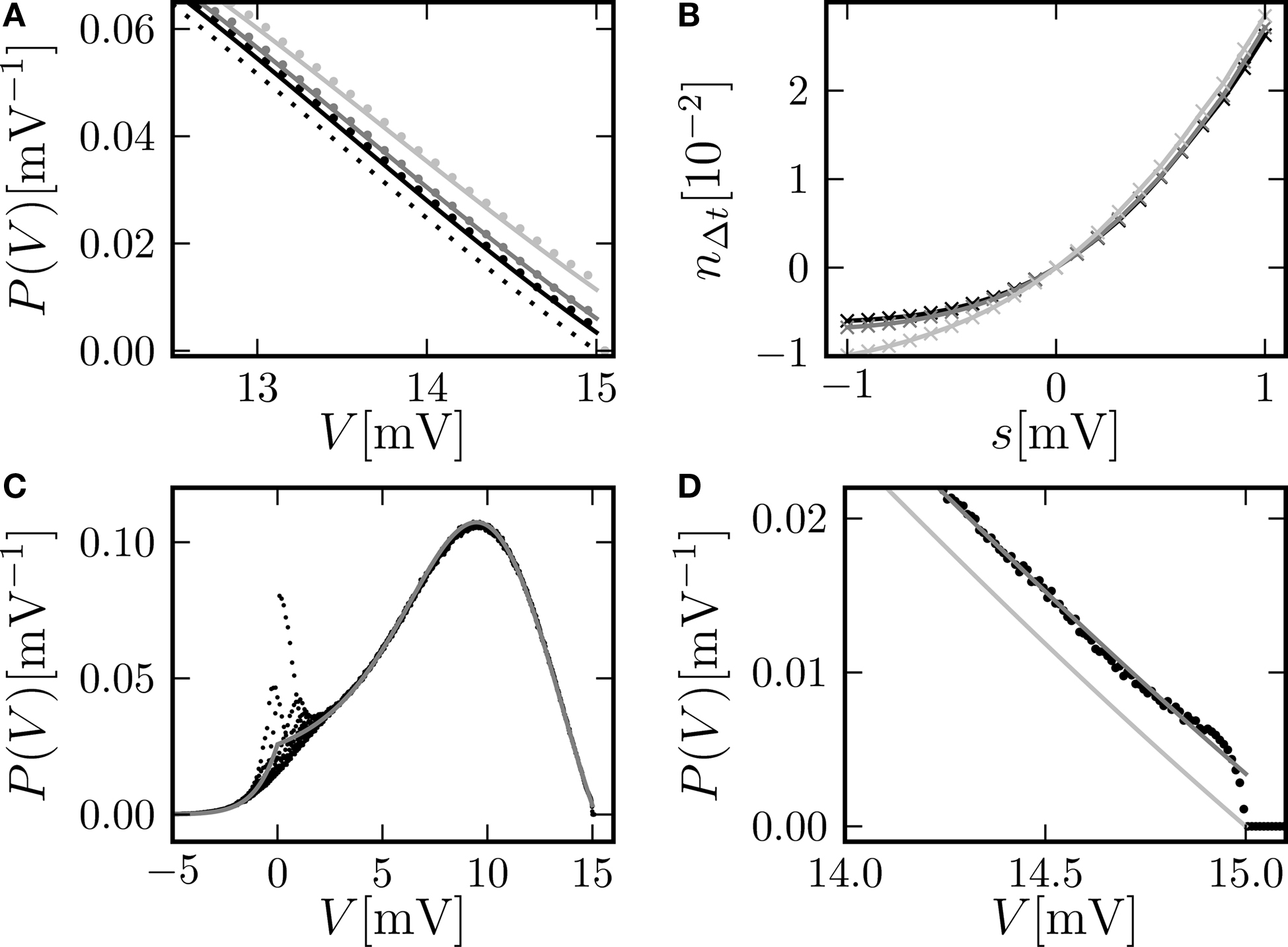
Figure 6. (A) Membrane potential distribution near the threshold for different simulation resolutions (black: h = 0.02 ms, gray: h = 0.1 ms, light gray: h = 0.5 ms). Analytic solution (Eq. 10) (solid gray and light gray lines), limit for h →0 of our theory (solid black line), direct simulation (dots), and theory of diffusion limit neglecting finite synaptic weights and discrete time (black dotted line) from Brunel (2000)
. (B) Direct simulation of the number of spikes  within the time window Δt = max (hi) = 0.5 ms excessing base rate caused by the perturbation for different simulation resolutions h (gray code as in A). Other parameters as in Figure 4
B. (C) Membrane potential distribution in continuous time for the same parameters as in Figure 2
A. Direct simulation in continuous time (black dots) and theory (gray) in the limit h → 0 (Helias et al., 2009
). (D) Zoom in of (C) near threshold (black dots, gray) and pure diffusion approximation (light gray) from Brunel (2000)
.
within the time window Δt = max (hi) = 0.5 ms excessing base rate caused by the perturbation for different simulation resolutions h (gray code as in A). Other parameters as in Figure 4
B. (C) Membrane potential distribution in continuous time for the same parameters as in Figure 2
A. Direct simulation in continuous time (black dots) and theory (gray) in the limit h → 0 (Helias et al., 2009
). (D) Zoom in of (C) near threshold (black dots, gray) and pure diffusion approximation (light gray) from Brunel (2000)
.In the limit of continuous time (Helias et al., 2009
) the density at threshold vanishes on a voltage scale given by the synaptic weight as shown in Figure 6
C,D. This limit can alternatively be obtained from the theory presented here by letting h → 0. Overall, our approach assuming the density to be discontinuous at threshold provides a better approximation than the classical diffusion limit, in which the density goes to 0 on the scale σ.
We present a novel treatment of both equilibrium and transient response properties of the integrate-and-fire neuron, where we extend the existing theory in two respects: Firstly, we allow for finite synaptic weights and secondly we incorporate the effect of time-discretization. We show that the appropriate absorbing boundary amounts to a Dirichlet boundary condition for the probability density assuming a finite value. The interesting special case of finite postsynaptic potentials in continuous time is taken care of in a separate manuscript (Helias et al., 2009
). These results can alternatively be obtained from the theory presented in the current work by taking the limit h → 0 in all equations presented. It turns out that the probability density in continuous time vanishes at threshold, but only on a very short voltage scale, such that qualitatively similar results hold for the response properties. Previously, low-pass filtering of synaptic noise has been demonstrated to have a similar effect on the membrane potential density (Brunel et al., 2001
). In our case, the consequences are comparable to the work cited: the neurons just below threshold can be caused to fire even by very small perturbations, and do not act as a low-pass filter, but rather respond instantaneously. In the absence of synaptic filtering, an instantaneous response has so far only been found for noise coded signals (Lindner and Schimansky-Geier, 2001
). Since our treatment of the instantaneous response is not based on perturbation theory, we are able to uncover its full non-linear dependence on the strength of the perturbation.
The novel analysis captures the equilibrium properties (probability density and mean firing rate) more accurately than the previous theory in the diffusion limit. Therefore, our theory allows for a better interpretation and understanding of simulation results. In particular it enables the quantification of artifacts due to time discretization, which have been discussed previously (Hansel et al., 1998
) in the context of artificial synchrony: The instantaneous response of the neuron model increases slightly with coarser discretization. To our knowledge, the treatment of an integrate-and-fire neuron by a density approach in discrete time is new as such. The description of the time evolution of a population of neurons in discrete time as a Markov process yields accurate figures for the mean firing rate and the equilibrium membrane potential density. The advantage of this method is that the computational costs are independent of the number of neurons in the population. If only the equilibrium and instantaneous response properties for a large number of non-interacting, identical neurons are required, this method is an effective replacement of direct simulation. However, both, the precision and the computational costs increase with finer discretization of the voltage axis. The complexity is dominated by the solution of an M × M system of linear equations, M being the number of discretization levels of the membrane voltage.
Our result can be applied to several problems of neural dynamics: Concerning recurrent networks, where the dynamics is replaced mostly by linear filters, our result suggests to extend the reduced model of a neuron by a linear filter plus an instantaneous response depending quadratically on the rectified input fluctuation with respect to baseline. The instantaneous non-linear response contributes to the peak at zero time-lag of the cross correlation function, which influences the transmission of correlated inputs by pairs of neurons to their output (Tetzlaff et al., 2003
; De la Rocha et al., 2007
). Spike timing dependent synaptic learning rules are sensitive to the shape of the correlation function between input and output of a neuron. The expansive increase of the immediate response with the size of the incoming synaptic event amounts to decrease of mean response time  of the neuron with respect to the incoming spike. This decrease can be detected by a spike timing dependent learning rule typically causing stronger synaptic potentiation at smaller latencies. Furthermore, it facilitates fast feed-forward processing observed in neural networks. The non-linearity between input and output transient is a property which might be useful to perform neural calculations (Herz et al., 2006
) and to increase the memory capacity of neural networks (Poirazi and Mel, 2001
).
of the neuron with respect to the incoming spike. This decrease can be detected by a spike timing dependent learning rule typically causing stronger synaptic potentiation at smaller latencies. Furthermore, it facilitates fast feed-forward processing observed in neural networks. The non-linearity between input and output transient is a property which might be useful to perform neural calculations (Herz et al., 2006
) and to increase the memory capacity of neural networks (Poirazi and Mel, 2001
).Moreover we observe aperiodic stochastic resonance for fast input transients here, which has previously been described for slow transients (Collins et al., 1996
): a certain range of noise amplitude promotes the modulation of the firing rate by these input signals. A qualitative understanding can readily be gained, observing that the membrane potential density near the threshold assumes a maximum at a certain noise level and hence alleviates the neuron’s response. One consequence is the noise-induced enhancement of the transmission of correlated activity through networks of neurons. Also, the response properties strongly affect the correlation between the efferent and afferent activity of a neuron, which influences spike timing dependent learning and effectively promotes the cooperative strengthening of synapses targeting the same neuron.
Our theory contains as a central assumption the applicability of a Fokker–Planck equation to describe the membrane potential distribution. Implicitly this assumes that all cumulants of the input current beyond order two vanish. As long as the firing rate of the incoming events is high and the synaptic weights are small, this is a good approximation. However, for low input rates and large synaptic weights these assumptions are violated and deviations are found. In particular the skewness of the distribution of synaptic jumps for asymmetric excitatory and inhibitory inputs induces deviations of the probability density obtained from our theory. A combination of our boundary condition with a more accurate treatment of the higher moments (Hohn and Burkitt, 2001
; Kuhn et al., 2003
) could provide better results in this case.
The second approximation in our theory is the behavior at threshold: We assume the density to vary on the scale σ in the whole domain. This approximation is satisfied to high precision far off the threshold and the reset, but especially close to these boundaries, modulations on the order of a synaptic weight and due to the deterministic evolution of the membrane potential within one time step become apparent. They are outside the scope of our current theory and the modulations at threshold have a noticeable effect on the accuracy of the predicted firing rate. Distributed synaptic weights should reduce this effect. The oscillations near the reset can be diminished by a different reset mechanism V ← V − Vθ proposed by Carl van Vreeswijk (private communication). Apart from a better agreement of the densities near reset, this has no noticeable effect on the results presented here. Fourcaud-Trocmé et al. (2003) and Naundorf et al. (2005)
found the spike generation mechanism to influence the response properties of neurons at high frequencies: they showed the response of the integrate-and-fire neuron to high-frequency sinusoidal currents in presence of filtered noise to be due to its hard threshold. Future work should investigate whether the immediate non-linear response observed here is also a property of neurons with more realistic thresholds, such as the exponential integrate-and-fire neuron (Fourcaud-Trocmé et al., 2003
).
Derivation of the Fokker–Planck Equation
To formalize the approach outlined in Section “Density Equation for the Integrate-and-Fire Neuron” we follow (Ricciardi et al., 1999
) and assume that the main contributions to the time evolution of the membrane potential distribution can be described by an infinitesimal drift and diffusion term. This is true, as long as the rate of incoming events is large  and postsynaptic potentials are small w ≪ Vθ − Vr. However, in the region near the threshold Vθ we treat the finite synaptic weights separately giving rise to the boundary condition described in Section “Boundary Condition at the Threshold and Normalization”. In addition to the stochastic input due to the incoming Poisson events, we assume the membrane potential to perform the deterministic change u(t), caused by an additional input. If E[] denotes the expectation value over realizations of the stochastic input, the infinitesimal drift becomes
and postsynaptic potentials are small w ≪ Vθ − Vr. However, in the region near the threshold Vθ we treat the finite synaptic weights separately giving rise to the boundary condition described in Section “Boundary Condition at the Threshold and Normalization”. In addition to the stochastic input due to the incoming Poisson events, we assume the membrane potential to perform the deterministic change u(t), caused by an additional input. If E[] denotes the expectation value over realizations of the stochastic input, the infinitesimal drift becomes
where we used  and introduced the abbreviations
  and the mean input
  The infinitesimal variance hence is
and introduced the abbreviations and the mean input The infinitesimal variance hence is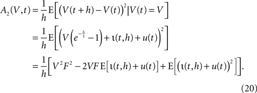
We use the explicit form of the second moments of the stochastic and the total input current, which are
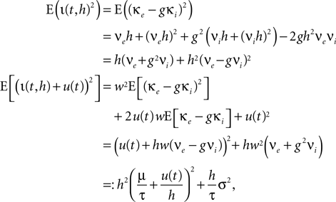
where we introduced the diffusion coefficient σ2: = τw2(νe + g2νi). So the infinitesimal variance becomes
Following Ricciardi et al. (1999)
we set up a diffusion equation for the membrane potential. The right hand side of this Fokker–Planck equation reads
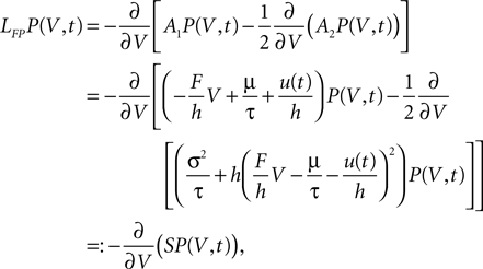
where we defined the probability flux operator S. Since we treat the problem in discrete time, a derivative with respect to time must be expressed as a finite difference. So the differential equation for the membrane potential distribution takes the form

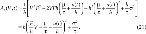
Letting the derivative on the right hand side act on A2 explicitly leads to
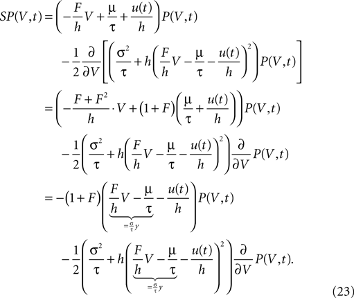
We find it convenient to introduce the dimensionless voltage  In addition, we express the probability density by a dimensionless density
 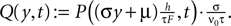 For the case
  the flux operator (Eq. 23) expressed in y and acting on Q becomes
In addition, we express the probability density by a dimensionless density For the case the flux operator (Eq. 23) expressed in y and acting on Q becomes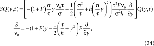
where we used 
General Solution of the Flux Differential Equation
To obtain the homogeneous solution of the Fokker–Planck equation (Eq. 22) we need to solve Eq. 5. Being a linear ordinary differential equation it has a particular (Qp) and a homogeneous solution (Qh), so the general solution can be written as

First, we determine the homogeneous solution (Eq. 6) satisfying SQh = 0.
We choose the integration constant C such that  According to Abramowitz and Stegun (1974)
we can express this as the Gauss hypergeometric series
According to Abramowitz and Stegun (1974)
we can express this as the Gauss hypergeometric series 
According to Abramowitz and Stegun (1974)
we can express this as the Gauss hypergeometric series 
So we will use in the following
Note that in the continuous limit h → 0 the homogeneous solution becomes a Gaussian  as in the diffusion limit. Its integral is also a hypergeometric series and we define
as in the diffusion limit. Its integral is also a hypergeometric series and we define
where for  the limit
  exists
the limit exists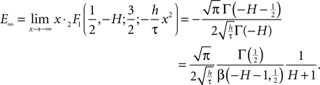
For large negative  (corresponding to
  ) this function turns into the known expression from the diffusion limit
(corresponding to ) this function turns into the known expression from the diffusion limit We determine the particular solution  of Eq. 5 that satisfies
  by variation of constants
of Eq. 5 that satisfies by variation of constants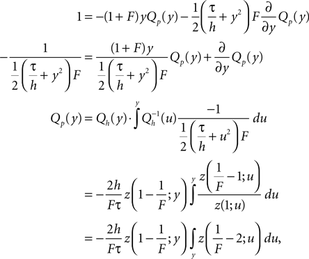
where the upper bound of the integral is yet arbitrary. Qp(y) fulfills SQp = ν0 by construction. In particular, here we choose the upper boundary as yθ to obtain Qp(yθ) = 0, which will be of advantage to determine the boundary condition at the threshold. To satisfy Eq. 5 and to be continuous at the reset together we choose
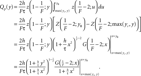
From the second to the third line, for numerical convenience we separated out the strongly divergent factor of Eq. 27 utilizing the identity (Abramowitz and Stegun, 1974
)
which yields (for  )
)
)
Boundary Condition at the Threshold
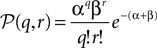
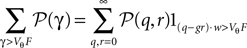
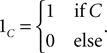
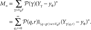
The numbers of incoming synaptic events κe, κi in a small time interval h are independently distributed with a Poisson distribution, so 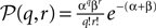 is the probability mass function to obtain q excitatory and r inhibitory synaptic events. The corresponding jump of the membrane potential is of size γ = (q − gr)w. The actual distribution of voltage jumps can hence be expressed as
is the probability mass function to obtain q excitatory and r inhibitory synaptic events. The corresponding jump of the membrane potential is of size γ = (q − gr)w. The actual distribution of voltage jumps can hence be expressed as
with
and
From the normalization condition it follows, that the membrane potential distribution  prior to arrival of synaptic inputs can be expressed by the distribution at the beginning of the time step P as
prior to arrival of synaptic inputs can be expressed by the distribution at the beginning of the time step P as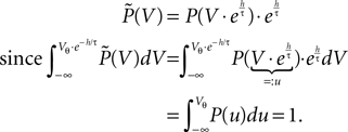
The boundary condition for the flux over the threshold is
We express P(V) by the dimensionless distribution Q(y) where we use
We solve for A to obtain
Using the explicit form for 𝒫(γ) (Eq. 29), we can replace the sums by
with
Taylor expansion of Q around the threshold and recurrence relation of derivatives
In order to evaluate Eq. 12, we can make use of the fact, that the width of the voltage jump distribution (Eq. 29) is typically small compared to the length scale σ on which the probability density function changes. So we can well approximate the probability density near the threshold by a Taylor polynomial of low degree. To this end, we derive a recurrence relation for the higher derivatives of P, or equivalently Q, here. The equilibrium probability density satisfies the flux differential equation (Eq. 5) with the flux operator given by Eq. 24 with  So, for yr ≤ y ≤ yθ, Q(y) satisfies
So, for yr ≤ y ≤ yθ, Q(y) satisfies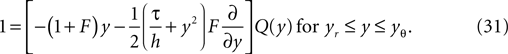
We define the shorthand qy which has the property
From this relation, we can recursively calculate the derivatives of Q as
It is easy to show by induction that the derivatives recurse for n ≥ 2 by

with an = 1 + nF
Due to linearity in Q of the differential equation (Eq. 24) and our choice Qp(yθ) = 0, we can split up the n-th derivative into the n-th derivative of the homogeneous solution, which is proportional to Q(yθ) and the n-th derivative of the inhomogeneous solution, which is independent of Q(yθ) and write it as Q(n)(yθ) = cn + dnQ(yθ) with

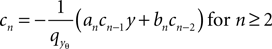
and
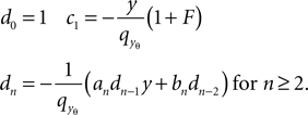
The expansion of Q around the threshold hence can be written as
where we identified the particular solution (Eq. 9) and the homogeneous solution (Eq. 26), respectively. Plugging the expansion Eq. 34 into Eq. 12 to obtain the boundary condition at the threshold, we get
with
Normalization
The probability density function has to be normalized
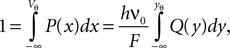
where we used the transformation (Eq. 3) to dimensionless quantities. Using the explicit form Eqs. 26 and 9 we obtain with Eq. 27
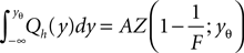
and with Eq. 28
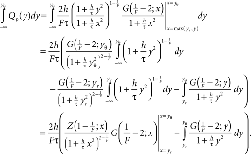
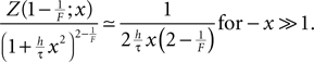
Both, the numerator and denominator in the boundary term go to 0 for large negative x. To improve numeric stability in this case, we found it necessary to replace the fraction by its approximation using l’Hopital’s rule. It yields
It allows us to calculate the mean firing rate ν0 of the neuron by
Numerical Solution of the Equilibrium Distribution
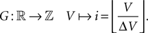
By discretizing the voltage range into bins where the size ΔV of a bin is chosen such that we can assume the probability density to be approximately constant within a bin and that ΔV integrally divides the synaptic weight w and gw, we can formulate the time evolution of the equilibrium distribution as a Markov Process on a discrete space. To this end we define the discretization operator G on the voltage axis as
The probability distribution P then becomes a vector  with the components
with the components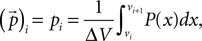
where we use νi = ΔV•i. Since we can assume the probability density to vanish for V → −∞, we can define a cutoff at some sufficiently negative voltage V− to obtain a finite dimensional space of dimension  In one time step, the voltage distribution decays, which is expressed by the linear operator D with
In one time step, the voltage distribution decays, which is expressed by the linear operator D with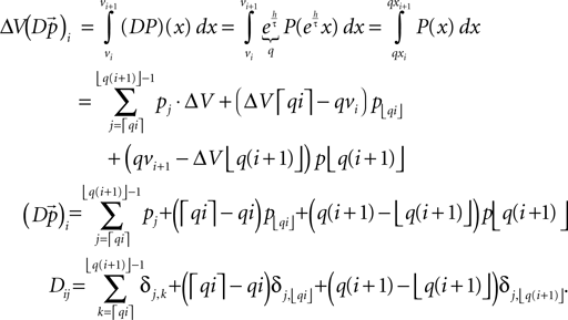
Similarly, we can express the effect of the input as a linear operator, given the jump distribution 𝒫(γ) Eq. 29, as
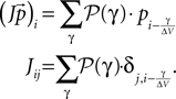
The threshold is performed by the operator T, which takes all states that are above threshold and inserts them at the reset
The evolution by one time step (as defined in Section “Density Equation for the Integrate-and-Fire Neuron”) is the composition of the three operations, D, J, and T
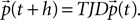
To find the stationary solution, we have to solve for the eigenvector to the eigenvalue 1 of TJD. This eigenvector exists because of the Perron–Frobenius theorem (MacCluer, 2000
), since our propagation matrix is column-stochastic Σj(TJD)ij = 1∀i. To additionally impose the constraint that the solution must be normalized, we add the equation ΔVΣipi = 1 to the first row, which we can write with Nij = ΔVδi,0 as
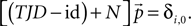
The stationary solution can then be found by numerically solving this linear equation for  We use Python (Python Software Foundation, 2008
) and the linear algebra package of SciPy (Jones et al., 2001
) for this purpose. The firing rate can be calculated from the equilibrium distribution
We use Python (Python Software Foundation, 2008
) and the linear algebra package of SciPy (Jones et al., 2001
) for this purpose. The firing rate can be calculated from the equilibrium distribution  from the probability mass exceeding the threshold in one time step
We use Python (Python Software Foundation, 2008
) and the linear algebra package of SciPy (Jones et al., 2001
) for this purpose. The firing rate can be calculated from the equilibrium distribution from the probability mass exceeding the threshold in one time step
Response of Firing Rate to Impulse like Perturbation of Mean Input
To calculate the DC-susceptibility of the firing rate with respect to μ we need to calculate  where ν0 is given by Eq. 14. With
  we only need to calculate
  Additionally, we note that
  to obtain
where ν0 is given by Eq. 14. With we only need to calculate Additionally, we note that to obtain
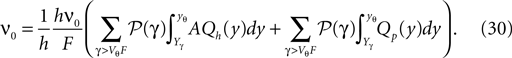
To calculate  we need the boundary condition (Eq. 30) which determines A
we need the boundary condition (Eq. 30) which determines A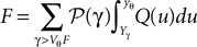
We differentiate with respect to μ and get

Since Q = AQh + Qp the integrand on the right hand side is
Using the explicit form of Qp (Eq. 9) its derivative with respect to μ is
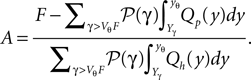
where we used that Yγ > yr and hence Qp depends on μ only through the upper bound yθ in the integral. This enables us to express the differentiated boundary condition (Eq. 39) as
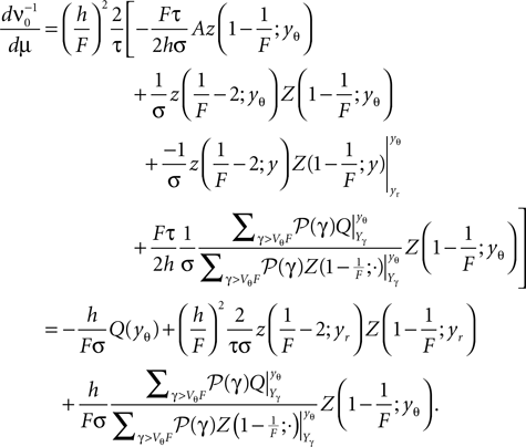
and we find
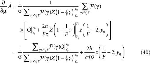
Inserting the expression (Eq. 40) into (Eq. 38) we can write
We can make use of the series expansion of Q at the threshold (Eqs. 34 and 35) to compute the numerator of in the last term as
and the denominator as
Numerical Implementation of Hypergeometric Series
The hypergeometric series F(a, b, c, z): = 2F1(a, b, c, z) is hard to evaluate for large absolute values of a and b = 1. Here we use the linear transformation formula (Abramowitz and Stegun, 1974
)
to reduce the magnitude of a. For b = 1 we obtain in particular
and
We use these two relations to define a recursive function which reduces the magnitude of a (using the first relation for a < 0 and the second for a > 0).
The authors declare that the research was conducted in the absence of any commercial or financial relationships that could be construed as a potential conflict of interest.
We would like to acknowledge very helpful discussions with Carl van Vreeswijk, Nicolas Brunel, and Benjamin Lindner, and we thank both reviewers for their constructive critique. Further, we gratefully appreciate ongoing technical support by our colleagues in the NEST Initiative. Partially funded by BMBF Grant 01GQ0420 to BCCN Freiburg, EU Grant 15879 (FACETS), DIP F1.2, Helmholtz Alliance on Systems Biology (Germany), and Next-Generation Supercomputer Project of MEXT (Japan).
Jones, E., Oliphant, T., and Peterson, P. (2001). SciPy: open source scientific tools for Python. http://www.scipy.org/Citing_SciPy
.
Python Software Foundation. (2008). The Python programming language. http://www.python.org
.