Département d’Informatique, École Normale Supérieure, Paris, France
“Brian” is a new simulator for spiking neural networks, written in Python (
http://brain.di.ens.fr
). It is an intuitive and highly flexible tool for rapidly developing new models, especially networks of single-compartment neurons. In addition to using standard types of neuron models, users can define models by writing arbitrary differential equations in ordinary mathematical notation. Python scientific libraries can also be used for defining models and analysing data. Vectorisation techniques allow efficient simulations despite the overheads of an interpreted language. Brian will be especially valuable for working on non-standard neuron models not easily covered by existing software, and as an alternative to using Matlab or C for simulations. With its easy and intuitive syntax, Brian is also very well suited for teaching computational neuroscience.
A reasonable question to ask is whether there is any need for another neural network simulator. There are now several mature simulators, which can simulate sophisticated neuron models and take advantage of distributed architectures with efficient algorithms (Brette et al., 2007
). Yet, many researchers in the field still prefer to use their own Matlab or C code for their everyday modelling work. It might be that currently available simulators do not fulfill the expectations of those users. Generally, what we expect from simulation software is that it should be able to run our specific model (flexibility) in a reasonable amount of time (efficiency). However efficiency is not only about the speed of simulations. The time it takes the user to implement the model is at least as important in many situations. For example, if it takes only 1 s to simulate a model with a given tool but 30 min to write the simulation script, one might prefer to use a tool which simulates the model in 10 s but for which the script can be written in 3 min. For those modelling situations, we only want the simulation software to be “reasonably fast”.
Brian is a new project (
http://brain.di.ens.fr
) to create a clock driven spiking neural network simulator with the goals of being easy to learn and use, highly flexible, and “reasonably fast”. It is ideally suited to rapid prototyping and refinement of networks of single compartment model neurons. Brian is written entirely in the Python programming language and will run on any platform that supports Python (i.e. almost all platforms). Users with a C compiler on their system can take advantage of a slight speed increase by opting to use certain core routines written in optimised C code, but these are strictly optional. Everything works the same without them. The way Brian works is that it is a Python package providing functions, classes and objects. It can be used either interactively using a Python shell, or as part of a Python program (module). Figure 1
shows a very simple Brian script. This script defines a randomly connected network of 4000 leaky integrate-and-fire neurons with exponential synaptic currents. This is Brian’s implementation of the current-based (CUBA) model network used as one of the benchmarks in Brette et al. (2007)
. The simulation takes 3–4 s on a typical PC, for 1 s of biological time (with dt = 0.1 ms). Figure 2
shows a more complicated example, illustrating many of the features of Brian.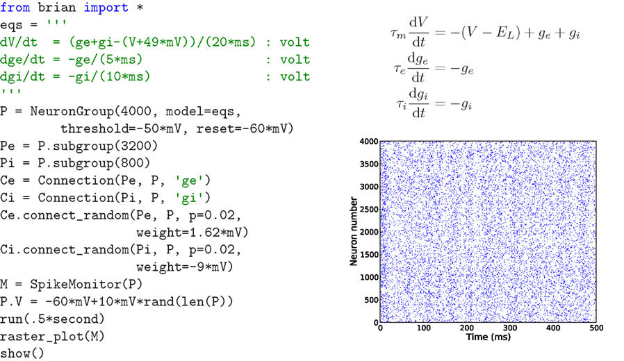
Figure 1. The CUBA network in Brian, with code on the left, neuron model equations at the top right and output raster plot at the bottom right. This script defines a randomly connected network of 4000 leaky integrate-and-fire neurons with exponential synaptic currents, partitioned into a group of 3200 excitatory neurons and 800 inhibitory neurons. The
subgroup() method keeps track of which neurons have been allocated to subgroups and allocates the next available neurons. The process starts from neuron 0, so Pe has neurons 0 through 3199 and Pi has neurons 3200 through 3999. The script outputs a raster plot showing the spiking activity of the network for a few hundred ms. This is Brian’s implementation of the current-based (CUBA) network model used as one of the benchmarks in Brette et al. (2007)
, based on the network studied in Vogels and Abbott (2005)
. The simulation takes 3–4 s on a typical PC (1.8 GHz Pentium), for 1 s of biological time (with dt = 0.1 ms). The variables ge and gi are not conductances, we follow the variable names used in Brette et al. (2007)
. The code :volt in the equations means that the unit of the variable being defined (V, ge and gi) has units of volts.
Figure 2. An example showing many of the features of Brian in action. The neuron model in this code follows a stochastic differential equation  . Here all the undefined symbols are constants except for
  which corresponds to the term
  The rest of the neuron model is defined by a custom reset function
. Here all the undefined symbols are constants except for which corresponds to the term xi in the code, and represents a white noise term The rest of the neuron model is defined by a custom reset function adaptive_threshold_reset which increases the value of Vt by a constant each time a neuron spikes (but never takes it above a fixed ceiling), and a custom threshold function lambda V,Vt:V>=Vt which defines the condition for a spike. The arguments to the custom reset function are a NeuronGroup object P (a population of neurons), and an array spikes containing the indices of the neurons in P that have spiked. Together these two custom functions define an adaptive threshold model. The option to specify custom functions makes Brian’s reset and threshold mechanism very flexible. The code also shows synaptic delays, and setting the synaptic weights with a custom function of (i, j), w*cos(2.*pi*(i-j)*1./100)). The output of the code shown is the raster plot in (B), with the value w=.5*mV. (A) shows w=.1*mV and (C) shows w=.65*mV. (D) shows the synaptic weight matrix for the w=.65*mV case. (E) and (F) show the values of V (solid blue) and Vt (dashed green) for the neuron with index 50 for the raster plots immediately above them ((B) and (C)) with w=.5*mV and w=.65*mV respectively.Background
One of the difficulties with current software for neural network simulation is the necessity to learn and use custom scripting languages for each tool: for example Neuron’s Hoc and NMODL (Carnevale and Hines, 2006
), NEST’s SLI (Gewaltig and Diesmann, 2007
), and Genesis’ SLI (Bower and Beeman, 1998
), the last two being different languages with the same name. This increases the learning curve and is less flexible than using an established language with strong support and development tools such as integrated development environments (IDEs), debuggers and profilers. Data analysis is either limited to those functions provided by the tool, or has to be carried out in another application such as Matlab, which can slow down the process of prototyping and refining models. Writing extensions to these tools can be rather difficult or somewhat inflexible, depending on whether extensions are written in the same language as the simulator itself.
To address this problem, there are projects in various stages of completion to provide Python interfaces for each of the tools mentioned above (see other chapters in this special issue). Because it is both easy and powerful, Python is rapidly becoming a standard tool in the field and in scientific computing more generally. In addition, the PyNN project is working to provide a unified Python interface to each simulator. These projects have considerable benefits. Users will only need to learn a single programming language rather than one or more for each tool, and that language is easy to learn, highly developed, very powerful, and has a large user base which provides excellent support and tools. A great deal of time can be saved working in just one environment, rather than having to switch back and forth between different applications and GUIs for developing models, running simulations and analysing data.
Brian complements these projects and has some additional benefits unique to it. Firstly, equations – differential equations in particular – can be defined at the highest level using standard mathematical notation (see Figures 1 and 2
). Brian does not restrict you to using standard models of neurons and synapses (although many are provided in the library), and neuron models based on new differential equations can be used without writing or compiling any code. Secondly, as Brian is written entirely in Python itself, it has all the advantages of the projects above and some additional ones. Integration with Python is tighter because the implementation is not in a separate language to the interface. This means that Brian can be used more flexibly, for example to write code which reads and modifies the variables of the simulation as it runs. Additionally, extensions to Brian are easy to write because everything is written in the same language.
Teaching
Brian was originally designed for research, but it would also make an ideal tool for teaching purposes. First of all, the Python language is extremely quick and easy to learn and the syntax allows code to be written very compactly, saving time and making it easier to present examples. Secondly, since Brian is written in pure Python, it works on almost every platform, so there are less compatibility issues for students with different hardware or operating systems. Finally, using Brian itself is very easy, and the core concepts and syntax of Brian code correspond very straightforwardly to neuroscientific concepts (see Figure 1
). Equations are specified using a familiar mathematical syntax, for example
eqs=quotidndV/dt=-V/tau:voltquotidn, where the only unfamiliar part of the syntax is the :volt term, which specifies that V has units of volts. Figure 1
shows that defining thresholds and resets is typically just a single keyword term such as threshold=-70*mV or reset=-55*mV, and creating groups of neurons is as simple as writing G=NeuronGroup(N,model).Features
Brian is a clock driven simulator, that is, all events take place on a fixed time grid t = 0, dt, 2dt, 3dt,…. Neuron models are normally defined by differential equations which can be arbitrary linear, nonlinear or stochastic, specified either by directly writing the equations in a string, by using standard equations such as leaky integrate-and-fire, or by building more complicated sets of equations using standard components such as K+ and Na+ currents. Both integrate-and-fire and Hodgkin–Huxley type models can be used. Multiple compartment models are possible, but at the moment they are neither particularly convenient nor efficient for more than a few compartments. For linear differential equations, Brian uses exact updates. For nonlinear differential equations, Euler (explicit) and exponential Euler (semi-implicit) methods are available (and more are planned).
Network connectivity can be built either directly by specifying connectivity per pair of neurons (i, j), or more efficiently with all-to-all or random connectivity, where the synaptic weights can be either single values or specified by a weight function f(i, j). Synaptic connections can include delays.
Network activity can be controlled in various ways. For spiking behaviour there are various standard models such as Poisson spiking neurons, and more direct control mechanisms can be used to specify spike times for a neuron with a list or Python function. While the simulation is running, all the variables of the simulator are directly accessible and this can be used for controlling almost any aspect of the simulation. The emphasis is on flexibility, and most aspects of the way Brian works can be overridden.
Basic support for short term plasticity and spike timing dependent plasticity is included. This will be standardised and made easier to use in later releases.
Brian also has a system for specifying quantities with physical dimensions, which makes things easier because variables can be entered without having to look up the scale defined for that variable by the simulator package, and is useful because it helps to catch hard to debug problems stemming from parameters or equations having inconsistent units (see Physical Units).
Finally, Brian is fairly efficient. Although Python is an interpreted language, it can still achieve speeds comparable to that of code written directly in C, and typically better than code written in Matlab. See the section “Simulation Speed” for a discussion of performance issues.
Brian is designed to be easy to use, flexible and reasonably fast. To achieve the first goal, Brian uses features of the Python programming language, in particular its extremely dynamic typing which allows code to be much simpler and more expressive. Flexibility in Brian stems from using a single high-level language for user code and the library itself, and from making differential equations a fundamental high-level data structure (see Background). For the third goal, Brian uses the strategy of vectorised code.
Brian makes considerable use of Python’s dynamic typing to make writing models easier, and to make the syntax concise and readable. So for example, in specifying a neuron model a thresholding procedure is required for producing spikes. This can be done by specifying a single number, a function, or a threshold object. In the first case, with the threshold specified by a single number Vt say, Brian infers the thresholding condition V ≥ Vt. In the second case, Brian examines the function provided. Consider a neuron model with variables
V and Vt, and the threshold specified as the function lambda V, Vt: V>=Vt (which is the Python expression for a function of two variables V and Vt which returns the value V>=Vt). In this case Brian examines the names of the arguments to the function and passes the appropriate values so that the code behaves as expected. This would be one way of providing a variable threshold condition (because Vt is a variable of the neuron model, and could evolve according to a differential equation or function of other variables for example). Another way is to provide a threshold object, either one of the standard types in the library, or a user-defined one by writing a class that derives from the Threshold class. The variable threshold condition above corresponds to the standard object VariableThreshold(quotidnVtquotidn) for example.Vectorising code is the strategy, familiar to users of Matlab, to minimise the amount of time spent in interpreted code compared to highly optimised array functions. This typically means trying to minimise the number of
for loops in code, and using data structures and algorithms that make this easier. Brian uses the NumPy package (see below) which has an array data type that makes, for example, the expression V[spikes]=Vr equivalent to but much faster than for i in spikes: V[i]=Vr. In Matlab this would be V(spikes)=Vr, and in many cases the NumPy syntax is very similar to the Matlab syntax making the transition between the two very easy. The issue of Brian’s speed and efficiency is covered in more detail in the section “Simulation Speed”.Brian uses the following standard Python packages: Numerical Python, which is designed for providing efficient array data structures and operations (NumPy,
http://www.scipy.org/NumPy
, Scientific Python, which extends NumPy to include more general algorithms for scientific work (SciPy, http://www.scipy.org
), and PyLab/Matplotlib for plotting (http://matplotlib.sourceforge. net/
).Worked Example
Figure 3
shows a slightly simplified version of the code in Figure 1
with diagrams showing schematically the meaning or function of each group of lines of code. Panels A through F illustrate lines of code, and Panel F, which corresponds to actually running the simulation, is composed of four sub-panels a through d which illustrate the four steps involved in each timestep dt of the simulation. We proceed to explain how this example works with reference to the figure.
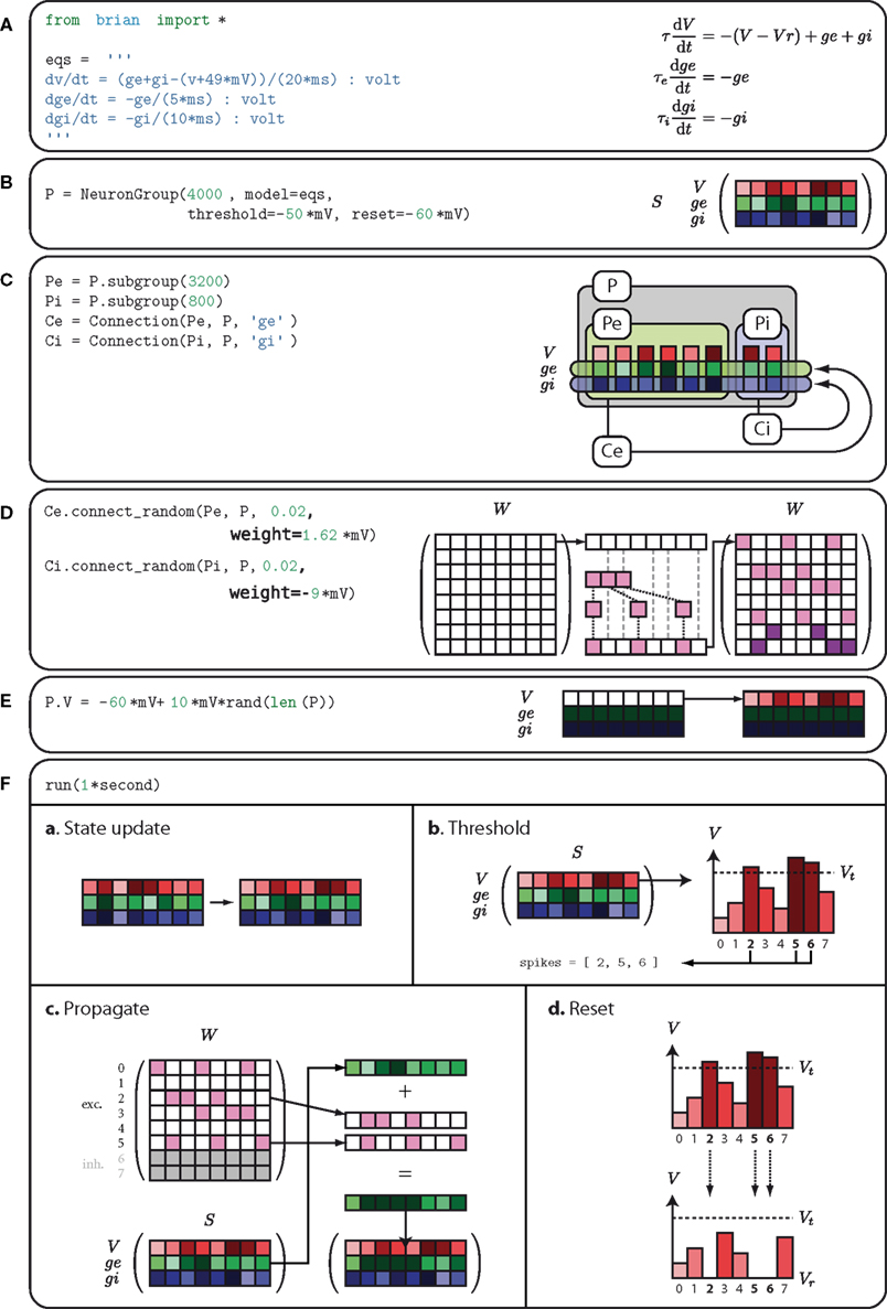
Figure 3. The code from Figure 1
expanded to show how Brian works internally. In (A), the equations for the model are defined. In (B), a group of 4000 neurons is created with these equations. In (C), the logical structure of the network is defined, partitioning the 4000 neurons into excitatory and inhibitory subgroups with corresponding connections to the whole group. In (D), the weight matrices for the excitatory and inhibitory connections are defined. In (E), the membrane potential is initialised uniformly randomly between reset and threshold values. In (F), the simulation is running, consisting of repeated applications of four operations each time step; (a) shows the update of the state matrix; (b) shows the thresholding operation; (c) shows the propagation of spikes; and (d) shows the reset operation.
A Firstly, the differential equations for the model are defined. This is illustrated in Panel A which shows the code which defines the equations and the equations in a more standard mathematical form. These equations will be used to define an integrate-and-fire neuron with exponential inhibitory and excitatory synapses with different time constants. The differential equation for V defines a leaky integrator with currents ge and gi. The variable ge is used for excitatory currents. When an excitatory spike arrives, the value of ge is increased instantaneously by a fixed amount. The inhibitory variable gi works similarly. Technically then, the full mathematical differential equations for the model would be:
where the superscripts indicate neuron indices, are the excitatory and inhibitory weight matrices, N = 4000 is the number of neurons, and
  is the time of the lth spike fired by neuron k. The spike propagation behaviour is defined in Panels C and D, see the description below.
are the excitatory and inhibitory weight matrices, N = 4000 is the number of neurons, and is the time of the lth spike fired by neuron k. The spike propagation behaviour is defined in Panels C and D, see the description below.B Having defined the differential equations, a group
P of 4000 neurons is created with these equations, a threshold mechanism set to fire spikes if V ≥ Vt = −50 mV, and a reset V ← Vr = − 60 mV. The diagram in Panel B shows Brian’s internal data structure for this group. It is a two-dimensional array or matrix S. At a given time the ith column of S holds the state variables for the ith neuron. Each row of the matrix is a vector of length 4000 of the values of a particular variable for all the neurons in the group.C The next step is to create the network structure. We create two subgroups
Pe and Pi of 3200 and 800 neurons respectively. The subgroup() method of the NeuronGroup object keeps track of which neurons have been allocated to subgroups and when called allocates the next available neurons. The process starts from neuron 0, so Pe has neurons 0 through 3199 and Pi has neurons 3200 through 3999. These two subgroups will be the excitatory and inhibitory neurons. In the diagram in Panel C, we have separated the columns of the state matrix S corresponding to each neuron. The excitatory and inhibitory subgroups are boxed and labelled Pe and Pi respectively. Next, excitatory and inhibitory connections Ce and Ci are created. The declaration of Ce specifies that the group Pe (the excitatory subgroup) should be connected to the variable ge (the excitatory current) of the group P (the whole group), and similarly for Ci. This means that when a neuron in Pe fires a spike, the variable ge will be increased for those neurons in P which the neuron in Pe synapses onto.D Having defined the logical network structure, we create the weight matrix itself. Each pair of neurons (i, j) are connected independently at random with probability 0.02. The excitatory synapses have weight 1.62 mV and the inhibitory ones have weight −9 mV (negative to make it inhibitory, and larger than the excitatory synapses as there are less inhibitory neurons). For efficiency, the random connectivity function constructs the sparse matrix row by row. For each row it generates a binomial random number k from B(N, p) which is the number of synapses in that row, and then randomly allocates those k synapses amongst the N possible target neurons, assigning them with equal fixed weight values. This process is illustrated in the diagram in Panel D.
E Now we prepare to actually run the simulation. The first step is to initialise the variables. At the start, all variables have the value zero. In Panel E, on the left hand side of the diagram, this is indicated by the V row being white (as 0 is much bigger than the threshold value which is negative), and the ge and gi rows being almost black. We leave the values of ge and gi as 0, and set V to be uniformly distributed between the reset and threshold values. The notation
P.V refers to the first row, the V row, of the state matrix S.F Finally, we run the simulation. Panel F shows the four operations executed each time step dt of the simulation: state update, threshold, spike propagation, and reset. In the state update phase (sub-panel a), the state matrix S is updated from t → t + dt, which as the differential equations are linear is just multiplication of S by a fixed matrix and addition of a fixed vector to each column of S. In the thresholding stage (sub-panel b), each value of V is simply compared to Vt and a list
Spikes of the indices of each of the neurons satisfying the condition is returned. In the propagation phase (sub-panel c), which is carried out separately for the excitatory and inhibitory connections, for each index i ∈ Spikes the ith row of W*, W [i,:], is added to the row vector corresponding to the variable g*, Finally, in the reset phase (sub-panel d), for each index i in Spikes, V is reset to Vr.This worked example shows the general anatomy of a Brian script: import the Brian package and define neuron models (Panel A); create groups of neurons (Panel B); create synaptic connections (Panels C and D); create monitors and other operations for recording data and controlling variables as a simulation runs (not shown in figure); initialise variables (Panel E); run the simulation (Panel F); and finally analyse and plot the data using any Python package (not shown in figure). Creating monitors and plotting output is not shown in Figure 3
but can be seen in Figure 1
. The lines
M=SpikeMonitor(P) and raster_plot(M) record and plot the spikes produced by the neurons in P. The raster_plot(M) function is part of Brian, but there are many Python packages which can be used for analysing and plotting data, including the ones used by Brian itself, NumPy, SciPy and Pylab/Matplotlib.Physical Units
Brian also features a system for specifying physical quantities with units. This is an independent package originally written for Brian but now available as a standalone package called Piquant (
http://piquant.sourceforge.net/
). It builds on the NumPy and SciPy packages, adding support for physical quantities. This has various benefits. It makes it possible to write code which syntactically and semantically expresses both the physical dimensions and scale of numbers. So for example, something like conductance=36*mS rather than conductance=36. In the latter case, the code alone does not express the value without knowing the standard scale for the software, and this often leads to errors which can be very hard to debug. In addition, because units retain their physical dimensions as well as their scale, accidentally writing something using the wrong units will cause an error (for example in Brian, differential equation with inhomogeneous units will raise an error).A quantity with physical units is a standard float value with an additional array of the indices of the seven fundamental SI units distance, mass, time, etc. The float value expresses the quantity at the standard SI scale, so that for example the float value of
1 *mV is 0.001. Operating on quantities with physical units is clearly more computationally demanding than operating on quantities without. To ameliorate this problem, Brian does two things. First of all, internal calculations done by Brian during a simulation only use the underlying float values, so that only initialisation code and custom functions use the units system. Secondly, Brian includes an option for switching the units system off globally. This only requires the addition of a single line of code to the top of a Brian program, and simply converts all the objects with units to their underlying float values. So for example with units turned off the symbol mS becomes the float value 0.001. The recommended usage is to leave the units system on when developing a model or when adding new code, and turning it off for longer and larger runs once the code is stable.Technical Details
The user specifies a model by providing the mathematical equations which define it. This can either be done directly by writing out the differential equations in full, or by building a set of equations using objects from the library (for things like ion channels or synapses). The former is useful in situations where there are not too many equations and where they are constantly being changed in the process of developing the model. The latter is useful in situations where the model is built from standard components and produces an unwieldy number of equations.
Given a final set of equations, Brian produces a  then the exact solution for the update step is X(t + dt) = eMdt(X(t) − B) + B, where eMdt is a constant matrix and B is a constant vector evaluated (numerically) at initialisation time (see Morrison et al., 2007
for a closed form method). Nonlinear equations are integrated by default with Euler updates, and the exponential Euler method (a semi-implicit method, MacGregor, 1987
) is also implemented for Hodgkin–Huxley models. The second-order Runge-Kutta method is also implemented. Stochastic differential equations are integrated with Euler updates (i.e., adding normally distributed random numbers every time step). Nonlinear equations given as text are compiled to Python functions at initialisation time, then used directly during the update phase with vector arguments [for example, x ← x + f(x)dt for a single state variable x and equation dx/dt = f(x)].
then the exact solution for the update step is X(t + dt) = eMdt(X(t) − B) + B, where eMdt is a constant matrix and B is a constant vector evaluated (numerically) at initialisation time (see Morrison et al., 2007
for a closed form method). Nonlinear equations are integrated by default with Euler updates, and the exponential Euler method (a semi-implicit method, MacGregor, 1987
) is also implemented for Hodgkin–Huxley models. The second-order Runge-Kutta method is also implemented. Stochastic differential equations are integrated with Euler updates (i.e., adding normally distributed random numbers every time step). Nonlinear equations given as text are compiled to Python functions at initialisation time, then used directly during the update phase with vector arguments [for example, x ← x + f(x)dt for a single state variable x and equation dx/dt = f(x)].
StateUpdater object. In general, this is an object that updates the state variables of a group of neurons in any way. For differential equations, it performs the integration step updating the state variables from times t to t + dt. Brian automatically inspects the equations to choose the most appropriate type of StateUpdater. For linear differential equations for example, updates are exact. More precisely, if the equations are then the exact solution for the update step is X(t + dt) = eMdt(X(t) − B) + B, where eMdt is a constant matrix and B is a constant vector evaluated (numerically) at initialisation time (see Morrison et al., 2007
for a closed form method). Nonlinear equations are integrated by default with Euler updates, and the exponential Euler method (a semi-implicit method, MacGregor, 1987
) is also implemented for Hodgkin–Huxley models. The second-order Runge-Kutta method is also implemented. Stochastic differential equations are integrated with Euler updates (i.e., adding normally distributed random numbers every time step). Nonlinear equations given as text are compiled to Python functions at initialisation time, then used directly during the update phase with vector arguments [for example, x ← x + f(x)dt for a single state variable x and equation dx/dt = f(x)].A
NeuronGroup object is created by specifying the number of neurons in the group and a model. A model requires a set of differential equations or a StateUpdater object, and can have optional thresholding and reset mechanisms. A Connection object is a mechanism for propagating spikes from one NeuronGroup to another. It is specified by an input group, an output group (which can be the same) and a target state variable. When a neuron in the input group fires a spike, the target state variable is increased for all the neurons in the output group to which that neuron is connected. This mechanism is very general and allows for all the standard types of synapses. Once a Connection object has been created, the actual connectivity of neurons can be specified in various ways. The main four ways are full connectivity, random connectivity, functionally specified connectivity (e.g. for spatial distributions) or by providing a connectivity matrix directly. The Connection methods Connect_random and Connect_full, for random and full connectivity respectively, take as their first two arguments the source and target neuron groups. This seems redundant because the Connection object knows the source and target groups, but the weight matrix can be constructed in blocks and the first two arguments to these methods can be subgroups of the groups specified in defining the Connection. In the present version, homogeneous synaptic delays can also be specified. Each neuron group stores a circular list of the last spikes over the required delay, each element of that list being an array of the indexes of neurons that spiked during one timestep. Spikes are then delivered in the same way as explained in the section “Worked Example” (Panel F).Python is an interpreted language, and although it is very fast there is an overhead for every Python operation. Brian can achieve very good performances by using the technique of vectorisation, similar to the same technique familiar to Matlab users. The idea is to replace loops by operations on large vectors, so that the interpretation overhead becomes negligible. Brian uses vectorisation for both the simulation and the construction of the model (e.g., initialisation of synaptic weights).
For example, for a single neuron i with state vector xi, the update step from xi(t) to xi(t + dt) might be xi(t + dt) = Mxi(t) + b for a matrix M and vector b. This operation is the same for every i so rather than looping through all the neurons carrying out the same operation, we write a state matrix S whose columns are the state vectors of each neuron. Now the loop carrying out the operation for each neuron i can be written in one operation, S(t + dt) = MS(t) + B (where B is a matrix with every column equal to b). The number of mathematical operations is the same, but the interpretation overhead is reduced from N interpretation operations for N neurons to 1 interpretation operation. Brian uses the NumPy package for these vectorised operations. NumPy is written in optimised C code, and for linear algebraic operations uses the Basic Linear Algebra Subprograms (BLAS) application programming interface (API). This means that NumPy can be combined with an implementation of the BLAS API that is optimised for the specific details of the processor it is running on. For large networks, the time spent on mathematical operations is much larger than the time spent on interpretation operations and so Brian is very efficient. For smaller networks, the interpretation overhead is much larger in proportion but in many situations it is not critical because the simulation time is shorter too. The least favourable scenario for Brian is the simulation of a small network for a long biological time.
Performance of Vectorised Simulations
In this section, we outline an analysis of Brian’s performance. A formula for the simulation time of a network with a clock-driven algorithm is given in Brette et al. (2007)
:
where cU is the cost of one update and cP is the cost of one spike propagation, N is the number of neurons, p is the number of synapses per neuron, F is the average firing rate and dt is the time step (the cost is for 1 s of biological time). If the simulation is fully vectorised, then interpretation can be included in this formula as a constant overhead cI per time step:
and the interpretation overhead becomes negligible when the network is large. In more detail, the update constant cI grows with the complexity of the model (in particular the number of variables) and the interpretation constant cI grows with the number of objects created, such as groups of neurons. Therefore, the strategy for running efficient simulations with Brian is to collect all neurons sharing the same differential equations in the same group. It is still possible to have heterogeneous groups in this way, for example the following code defines a group of 100 integrate-and-fire neurons with membrane time constants between 5 and 30 ms:
Here
tau becomes a state variable instead of a parameter. The same method can be used to obtain the results of a simulation for different parameter values. Note that with this change the differential equation becomes nonlinear with respect to the two variables; equations are then integrated with an approximation scheme (Euler by default). A mechanism for declaring state variables to be constant so that the above equation would be considered linear and integrated with exact matrix updates (one matrix for each parameter value) is in preparation for a future release of Brian.In many cases, the initialisation can also be vectorised. For example, the following instruction connects all pairs of neurons of a group with a distance-dependent weight (the topology is a ring):

The program builds the weight matrix row by row by calling the weight function with arguments (i, j) where i is the row number and j is the vector (0, 1,…, N − 1). Thus, the matrix is constructed with N vector-based operations, in a way that is transparent to the user. This is made possible by the fact that Python is a dynamically typed language (functions do not need to specify the type of their arguments in their definition).
Comparison with C and Matlab
In this section, we compare the empirical performance of Brian with that of C and Matlab. We compare absolute performance and, since it was always the fastest, times relative to C. The C code was always compiled with the heaviest optimisations possible, the
-03 switch with the gcc compiler. Brian was always run with the optional compilation switch on, and unit checking turned off. This means that certain key routines (the thresholding operation and the spike propagation phase) were written in C to avoid the Python overheads. These key operations are very generic, and so having them written in C rather than pure Python does not affect the flexibility of Brian as a whole. Note that this compilation switch is optional, and on a system without a C compiler installed Brian will use alternative versions of these core routines which are slightly slower but still very usable. Typically, running Brian with pure Python only takes about 25–50% longer than with the C routines. In the following benchmarks, times were computed by running each set of parameters 10 times and taking only the 7 best times, which helps to remove outliers where performance is degraded due to the operation of an unrelated process running on the system. The comparisons shown were obtained using a 2.33 GHz Intel Xeon processor with 2 GB RAM running on Windows XP. The version of NumPy used was 1.1.1 with the default BLAS linear algebra package. Using a custom build of NumPy with a BLAS package tuned for the particular CPU architecture would give better performance. The source code for the comparisons is available on request.The first benchmark we consider is a modified version of the CUBA network presented above in Figures 1 and 3
. This is a network of linear differential equations, and Brian does exact updates for the state matrix for t → t + dt which amounts to a matrix multiplication. We used the same mechanism exactly for the C and Matlab code. In all cases, the connection matrix uses a sparse matrix data structure implemented in effectively the same way.
We first modify the network so that instead of random connectivity with each pair of neurons connected with probability 0.02, the probability is p/N, where N is the number of neurons, making an average of p synapses per neuron independent of N. This guarantees that the firing rate of an individual neuron is independent of N. According to the calculations in the section “Performance of Vectorised Simulations” then, the computation time as a function of N should be proportional to N. Figure 4
shows the times for this network. You can see that the performance of Brian is better than Matlab, but not as good as C. You can also see that as N increases, the relative performance of Brian compared to C improves. This is because the Python overheads are a fixed cost independent of N. At N = 32,000, Brian takes approximately 2.4 times as long as C, and we would expect that this ratio would improve further for larger N. For this N, Matlab takes approximately seven times as long as C.
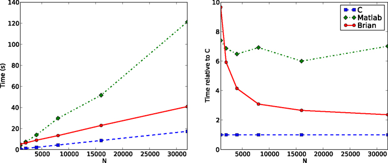
Figure 4. Computation time for the CUBA network using Brian, C and Matlab. This version of the CUBA network uses a fixed 80 synapses per neuron, and a varying number of neurons N. The figure on the left shows the absolute time on the test machine. The figure on the right shows the time compared to the C code. Theoretically, we would expect O(N) computation time (see Performance of Vectorised Simulations).
The next benchmark is the same CUBA network, but this time with all synapses removed. Performance in general is largely dominated by two factors: the state update phase, and the spike propagation phase. This benchmark gives an idea of how performance for the state update phase alone scales. Figure 5
shows the comparison. For large N, Brian takes around twice as long as C, and Matlab about four times as long. The jump in the times for Brian going from N = 16,000 to N = 32,000 may be due to CPU cache behaviour.
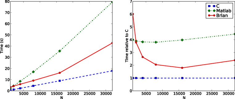
Figure 5. Computation time for the CUBA network if all synapses are removed. This largely demonstrates the performance for the state update step, which in this case is a matrix multiplication.
The next benchmark uses a fixed N, but varies the parameter we, the excitatory synaptic weight. Increasing this increases the firing rate. Figure 6
shows the comparison. For the range of we shown, leading to a range of firing rates from about 5 Hz to about 25 Hz, the times appear to grow at a similar rate for each of C, Matlab and Brian.
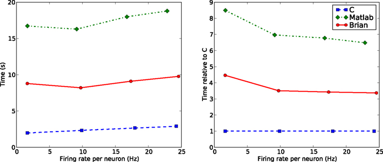
Figure 6. Computation time for the CUBA network with on average p = 500 synapes per neuron and N = 4000 at different firing rates. The parameter we, the excitatory weight, was varied between 1.62 and 4.8 mV which had the effect of varying the firing rate between about 5 Hz and about 25 Hz. This shows how performance scales with the number of spikes. Here the firing rates as well as the times are averaged over the seven fastest trials, as firing rates vary from trial to trial. Note that times due to spiking depend on both the firing rate and the number of synapses per neuron.
In conclusion, Brian is mostly around two to four times slower than C code for the typical network considered, and Matlab is around seven times slower. For smaller networks, Brian is slower than this, and for larger networks, we expect Brian to be faster than this. This seems like a reasonable trade off, given that smaller networks tend to take less time to run in absolute terms than larger networks.
Brian has been developed for quickly coding models of spiking neural networks in everyday situations. It is easy to learn, intuitive and flexible, which also makes it ideal for teaching. Although it is written in an interpreted language, it remains computationally efficient in many situations thanks to vectorised algorithms. It is however not currently designed for very large scale simulations which require clusters of computers, or for detailed biophysical models with complex morphologies.
Community
Brian is open source, and we are following the open source strategies of code reuse and interoperability. To make the development effort lighter and support easier, we chose to use existing packages and components as much as possible, and only write what is necessary on top of that. In writing Brian, we have used the NumPy, SciPy and PyLab/Matplotlib packages. There is a PyNN module for Brian currently in development, through which Brian will support open standards such as NeuroML (Goddard et al., 2001
) and other XML description standards (Cannon et al., 2007
).
We would also encourage others to make their code written with Brian accessible to others. Complete models can be posted to ModelDB (Hines et al., 2004
), and in addition there is the new “Computational Neuroscience Cookbook” project hosted on the NeuralEnsemble website (
http://neuralensemble.org/cookbook
). The idea of the cookbook is for submission of fragments of code which can be cut and pasted into others’ code. Finally, we encourage others to contribute to the Brian project itself (http:// brian.di.ens.fr/contribute.html
).Future Work
In the near future, our priorities for improving Brian are increasing the efficiency of Brian simulations and adding more modelling features. Specifically, we have started using the parallel processors present in modern graphics cards (GPU, Graphics Processing Unit) to improve the speed of Brian simulations with no additional work from the user (Luebke et al., 2004
). These can be used as parallel coprocessors for vectorised calculations (Cummins et al., 2008
). On the modelling side, we are focusing our efforts on synaptic plasticity. It is already possible to simulate spike timing dependent plasticity (STDP, as in e.g. Song et al., 2000
) and short term plasticity (STP; Tsodyks and Markram, 1997
) with the current mechanisms implemented in Brian (since these are defined as differential equations with resets in those references, see Morrison et al., 2008
for a review of plasticity rules), and we are working on making it as flexible and simple to use as possible.
The authors declare that the research was conducted in the absence of any commercial or financial relationships that could be construed as a potential conflict of interest.
This work was partially supported by the European Union (Visiontrain, a Marie Curie Research Training Network) and by the French ANR (ANR-RIAM Wired Smart). The authors would like to thank all those who tested early versions of Brian and made suggestions for improving it.
Brette, R., Rudolph, M., Carnevale, T., Hines, M., Beeman, D., Bower, J. M., Diesmann, M., Morrison, A., Goodman, P. H., Harris, F. C., Zirpe, M., Natschläger, T., Pecevski, D., Ermentrout, B., Djurfeldt, M., Lansner, A., Rochel, O., Vieville, T., Muller, E., Davison, A. P., Boustani, S. E., and Destexhe, A. (2007). Simulation of networks of spiking neurons: a review of tools and strategies. J. Comput. Neurosci. 23, 349–398.
Cummins, G., Adams, R., and Newell, T. (2008). Scientific computation through a GPU. In Proceedings of the Southeastcon 2008, an IEEE conference, Huntsville, AL, pp. 244–246. http://ieeexplore.ieee.org/xpl/freeabs_all.jsp?arnumber=4494293