1
Brain Mapping Unit, Department of Psychiatry, University of Cambridge, Cambridge, UK
2
Behavioural and Clinical Neurosciences Institute, University of Cambridge, Cambridge, UK
3
Institute for Mathematical Sciences, Imperial College, London, UK
4
Melbourne Neuropsychiatry Centre, Department of Psychiatry, University of Melbourne, VIC, Australia
5
GSK Clinical Unit Cambridge, Addenbrooke’s Hospital, Cambridge, UK
The idea that complex systems have a hierarchical modular organization originated in the early 1960s and has recently attracted fresh support from quantitative studies of large scale, real-life networks. Here we investigate the hierarchical modular (or “modules-within-modules”) decomposition of human brain functional networks, measured using functional magnetic resonance imaging in 18 healthy volunteers under no-task or resting conditions. We used a customized template to extract networks with more than 1800 regional nodes, and we applied a fast algorithm to identify nested modular structure at several hierarchical levels. We used mutual information, 0 < I < 1, to estimate the similarity of community structure of networks in different subjects, and to identify the individual network that is most representative of the group. Results show that human brain functional networks have a hierarchical modular organization with a fair degree of similarity between subjects, I = 0.63. The largest five modules at the highest level of the hierarchy were medial occipital, lateral occipital, central, parieto-frontal and fronto-temporal systems; occipital modules demonstrated less sub-modular organization than modules comprising regions of multimodal association cortex. Connector nodes and hubs, with a key role in inter-modular connectivity, were also concentrated in association cortical areas. We conclude that methods are available for hierarchical modular decomposition of large numbers of high resolution brain functional networks using computationally expedient algorithms. This could enable future investigations of Simon’s original hypothesis that hierarchy or near-decomposability of physical symbol systems is a critical design feature for their fast adaptivity to changing environmental conditions.
Almost 50 years ago, Herbert Simon wrote an essay entitled “The architecture of complexity” (Simon, 1962
). In this prescient analysis, he argued that most complex systems, such as social, biological and physical symbolic systems, are organized in a hierarchical manner. He introduced the notion of “nearly-decomposable systems”, i.e. systems where elements have most of their interactions (of any kind) with a subset of elements in some sense close to them, and much less interaction with elements outside this subset. In mainstream contemporary parlance, Simon’s near-decomposability is closely analogous to the concept of topological modularity: nodes in the same module have dense intra-modular connectivity with each other and sparse inter-modular connectivity with nodes in other modules (Newman, 2004
, 2006
). Simon argued that near-decomposability was a virtually universal property of complex systems because it conferred a very important evolutionary or adaptive advantage. Decomposability, or modularity, accelerates the emergence of complex systems from simple systems by providing stable intermediate forms (component modules) that allow the system to adapt one module at a time without risking loss of function in other, already-adapted modules.
Our understanding of complexity has progressed considerably since that time, partly due to the availability of large data-sets that now allow us to explore empirically the architecture of complex systems and thereby to feedback on theoretical considerations (Strogatz, 2001
; Amaral and Ottino, 2004
). Many complex systems can be represented using tools drawn from graph theory as networks of nodes linked by edges. Such networks have been used to represent a broad variety of systems, ranging from genetic and protein networks to the World Wide Web. The huge size of some of these systems (∼10 billion nodes in the WWW) has driven the development of new statistical tools in order to characterize their topological properties (Newman, 2003
).
A quantity called modularity has been introduced in order to measure the decomposability of a network into modules (Guimerà et al., 2004
; Newman and Girvan, 2004
). Modularity can be used as a merit function to find the optimal partition of a network. The resulting partition has been shown to reveal important network community structures in a variety of contexts, e.g. the global air transportation network (Guimerà et al., 2005
) and gene expression interactomes (Oldham et al., 2008
) are two diverse examples of complex systems with topological modularity. However, in systems having an intrinsic hierarchical structure, finding a single partition is not satisfactory. Several approaches have therefore been proposed in order to allow for more flexibility and to uncover communities at different hierarchical levels. Among those multi-scale approaches, there are algorithms searching for local minima of the modularity landscape (Sales-Pardo et al., 2007
) or modifying the adjacency matrix of the graph in order to change its typical scale (Arenas et al., 2008
). Another class of methods consists in modifying modularity by incorporating in it a resolution parameter (Reichardt and Bornholdt, 2006
). This allows one to “zoom in and out” of a modular hierarchy in order to find communities on different levels; for example, the resolution parameter can be interpreted as the time scale of a dynamical process unfolding on a network (Lambiotte et al., 2009
).
There is already strong evidence that brain networks have a modular organization; see Bullmore and Sporns (2009)
for review. Some support comes from non-human data, like the anatomical networks in felines and primates (Hilgetag et al., 2000
) or functional networks in rodents (Schwarz et al., 2008
). Recently, human neuroimaging studies have also provided evidence for comparable modular organization in both anatomical (Chen et al., 2008
) and functional (Ferrarini et al., 2009
; Meunier et al., 2009
) brain networks. However, a limitation of these previous neuroimaging studies has been the computational time required to derive a modular decomposition (Brandes et al., 2006
), thus limiting the size of the networks under study. In addition, these studies were limited to studying modularity at one particular level of community structure, neglecting consideration of possible sub-modular communities at lower levels. Finally, it has been a taxing problem to quantify the topological similarity between two or more modular decompositions, with most investigators simply examining modularity on the basis of an averaged connectivity matrix estimated from a group of individuals.
In this study, we report on progress towards addressing each of these issues. We applied a recently developed, computationally efficient algorithm (Blondel et al., 2008
) to derive a hierarchical, modular decomposition of human brain networks measured using functional magnetic resonance imaging (fMRI) in 18 healthy volunteers. By providing rapid decomposition, the algorithm enabled us to study the modular structure of whole brain networks on a larger scale (thousands of equally sized nodes) than previously possible (tens of differently sized nodes), with concomitant improvements in the spatial or anatomical resolution of the network, while simultaneously avoiding biases associated with using a priori anatomical templates that are inevitably somewhat arbitrary in their definition of regions-of-interest (Tzourio-Mazoyer et al., 2002
). Thus, the method enabled rapid, high-resolution, hierarchical modular decomposition of brain functional networks constructed from individual fMRI datasets. In addition, we present a method for comparing the similarity or mutual information between two modular community structures obtained for different subjects, and use it to identify the single, “most representative” subject whose brain network modularity was most similar to that of all the other networks in a sample of 18 healthy participants.
Experimental Data
Study sample
Eighteen right-handed healthy volunteers (15 male, 3 female) were recruited from the GlaxoSmithKline (GSK) Clinical Unit Cambridge, a clinical research facility in Addenbrooke’s Hospital, Cambridge, UK. All volunteers (mean age 32.7 years ± 6.9 SD) had a satisfactory medical examination prior to study enrolment and were screened for any other current Axis I psychiatric disorder using the Structured Clinical Interview for the DSM-IV-TR Axis I Disorders (SCID). Participants were also screened for normal radiological appearance of structural MRI scans by a consultant neuroradiologist, and female participants were screened for pregnancy. Urine samples were used to confirm abstinence from illicit drugs and breath was analysed to ensure that no participant was under the influence of acute alcohol intoxication. All volunteers provided written informed consent and received monetary compensation for participation. The study was reviewed and approved by the Cambridge Local Research Ethics Committee (REC06/Q0108/130; PI: TW Robbins).
Functional MRI data acquisition
Whole-brain echoplanar imaging (EPI) data depicting BOLD contrast were acquired at the Wolfson Brain Imaging Centre, University of Cambridge, UK, using a Siemens Magnetom Tim Trio whole body scanner operating at 3 T with a birdcage head transmit/receive coil. Gradient-echo, EPI data were acquired for the whole brain with the following parameters: repetition time = 2000 ms; echo time = 30 ms, flip angle = 78°, slice thickness = 3 mm plus 0.75 mm interslice gap, 32 slices parallel to the inter-commissural (AC-PC) line, image matrix size = 64 × 64, within-plane voxel dimensions = 3.0 mm × 3.0 mm.
Participants were asked to lie quietly in the scanner with eyes closed during the acquisition of 300 images. The first four EPI images were discarded to account for T1 equilibration effects, resulting in a series of 296 images, of which the first 256 images were used to estimate wavelet correlations.
Functional MRI data preprocessing
The images were corrected for motion and registered to the standard stereotactic space of the Montreal Neurological Institute EPI template image using an affine transform (Suckling et al., 2006
). Time series were then extracted using a whole brain, high resolution, regional parcellation of the images, implemented in the following manner; see Figure 1
A. First, a binarized version of a commonly used template image (Tzourio-Mazoyer et al., 2002
) was used as a broad grey matter mask. Second, each 8 mm3 voxel in this mask was downsampled by a factor of 4 such that each equally sized region in the parcellation comprised 4 × 4 × 4 voxels of the original image. This initial parcellation included some regions of the image which were not largely representative of grey matter: these were excluded from further analysis by applying the criteria that each region must be at least 50% overlapping with the grey matter mask and must contain at least 80% voxels having BOLD signal (defined operationally as mean signal intensity >50). To be included in the definitive parcellation scheme (which comprised 1808 regional nodes), a region had to satisfy these two inclusion criteria for every individual dataset in the sample.
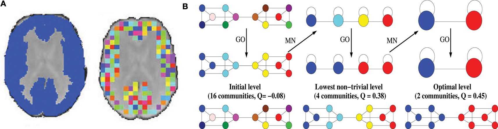
Figure 1. Methods. (A) Downsampled template. Starting from a binary version of the AAL template (left), the downsampling procedure will produce a template of small (64 voxels), equal size regions covering the original template (right). (B) Illustration of the Louvain method on a simple hierarchical graph. The algorithm starts by assigning a different module to each node (16 modules of single nodes). The method then consists of two phases that are repeated iteratively. The first phase is a greedy optimization (GO) where nodes adopt the community of one of their neighbours if this action results in an increase of modularity (typically, the community of the neighbour for which the increase is maximal is chosen). The second phase builds a meta-network (MN) whose nodes are the communities found in the first phase. We denote by “pass” a combination of these two phases. The passes are repeated until no improvement of modularity is possible and the optimal partition is found. When applied on this graph, the algorithm first finds a lowest non-trivial level made of four communities. The next level is the optimal level and is made of two communities.
The mean time series of each region was extracted and wavelet-filtered using Brainwaver R package
1
(Achard et al., 2006
; Achard and Bullmore, 2007
). The wavelet correlation coefficient was estimated for each of four wavelet scales between each pair of nodes, resulting in a {1808 × 1808} association matrix, or frequency-dependent functional connectivity matrix, for each wavelet scale in the overall frequency range 0.25–0.015 Hz. In what follows, we will focus on results at wavelet scale 3, subtending a frequency interval of 0.06–0.03 Hz.
This choice of frequency interval was guided by the fact that prior work on resting-state fMRI functional connectivity has found that the greatest power in connectivity occurs in frequency bands lower than 0.1 Hz (Cordes et al., 2001
). However, analysing very low frequency scales in limited time series such as those acquired with fMRI can reduce precision in estimating inter-regional wavelet correlations (Achard et al., 2006
). So scale 3 was chosen for the focus of this study as representing a reasonable compromise between retaining sufficient estimation precision while measuring low frequency network properties.
Each association matrix was thresholded to create an adjacency matrix A, the ai,jth element of which is either 1, if the absolute value of the wavelet correlation between nodes i and j, wi,j, exceeds a threshold value τ; or 0, if it does not. We have chosen here to take a high threshold, leading to very sparse networks comprising 8000 edges, i.e. with a connection density of 0.5% of all possible edges in a network of this size. Modularity of neuroimaging networks is typically greater (Meunier et al., 2009
), and computational costs are lower, when the networks are more sparsely thresholded. Up to 10% of nodes were disconnected from the rest of the network at this threshold.
Graph Theoretical Analysis
Hierarchical modularity
In recent years, many methods have been proposed to discover the modular organization of complex networks. A key step was taken when Girvan and Newman popularized graph-partitioning problems by introducing the concept of modularity. Modularity is by far the most widespread quantity for measuring the quality of a partition 𝒫 of a network. In its original definition, an unweighted and undirected network that has been partitioned into communities has modularity (Newman and Girvan, 2004
):
where A is the adjacency matrix of the network; m is the total number of edges; and  is the degree of node i. The indices i and j run over the N nodes of the graph. The index C runs over the modules of the partition 𝒫. Modularity counts the number of edges between all pairs of nodes belonging to the same community or module, and compares it to the expected number of such edges for an equivalent random graph. Modularity therefore evaluates how well a given partition concentrates the edges within the modules.
is the degree of node i. The indices i and j run over the N nodes of the graph. The index C runs over the modules of the partition 𝒫. Modularity counts the number of edges between all pairs of nodes belonging to the same community or module, and compares it to the expected number of such edges for an equivalent random graph. Modularity therefore evaluates how well a given partition concentrates the edges within the modules.A popular method for discovering the modules of a network consists in optimizing modularity, namely in finding the partition having the largest value of 𝒬. However, it is typically impossible computationally to sample modularity exhaustively by enumerating all the possible partitions of a network into communities. Several heuristic algorithms have therefore been proposed to provide good approximations, and so to allow for the analysis of large networks in reasonable times. The computational expediency of the algorithm has become a crucial factor due to the increasing size of the networks to be analysed.
More recently, methods to study hierarchical modularity, also called nested modularity, have been introduced (Sales-Pardo et al., 2007
; Arenas et al., 2008
; Rosvall and Bergstrom, 2008
). In this case, each module obtained at the partition of the highest level can further be decomposed into sub-modules, which in turn can be decomposed into sub-submodules, and so on. Here, we will use a multi-level method which was introduced very recently in order to optimize modularity (Blondel et al., 2008
); see Figure 1
B. The primary advantages of this method are that it unfolds a complete hierarchical community structure for the network and outperforms previous methods with respect to computation time. This so-called “Louvain method” takes advantage of the hierarchical organization of complex networks in order to facilitate the optimization. The algorithm starts by assigning a different module to each node of the network. The initial partition of the network is therefore made of N communities. It then consists of two phases that are repeated iteratively. The first phase consists in a greedy optimization where nodes are selected sequentially in an order that has been randomly assigned. When a node is selected, it may leave its community and adopt a community which is in its direct neighbourhood, but only if this change of community leads to an increase of modularity (GO on Figure 1
B). The second phase builds a new network whose meta-nodes are the communities found in the first phase (MN on Figure 1
B). Let us denote by “pass” a combination of these two phases. These passes are repeated iteratively until a maximum of modularity is attained and an optimal partition of the network into communities is found. By construction, the meta-nodes, or intermediate communities, are made of more nodes at subsequent passes. The optimization is therefore done in a multi-scale way: among adjacent nodes at the first pass, among adjacent meta-nodes at the second pass, etc. The output of the algorithm is a set of partitions, one for each pass. The optimal partition is the one found at the last pass. It has been shown on several examples that modularity estimated by this method is very close to the optimal value obtained from slower methods (Blondel et al., 2008
). Intermediate partitions can also be shown to be meaningful and to correspond to communities at intermediate resolutions (see Section “Discussion”). In the following, we will call “lowest non-trivial level” the partition found after the first pass.
Node roles
Once a maximally modular partition of the network has been identified, it is possible to assign topological roles to each node based on its density of intra- and inter-modular connections (Guimerà and Amaral, 2005a
,b
; Guimerà et al., 2005
; Sales-Pardo et al., 2007
).
Intra-modular connectivity is measured by the normalized within-module degree,
where  is the number of edges connecting the ith node to other nodes in the nth module,
  is the average of
  over all nodes in the module n, and
  is the standard deviation of the intra-modular degrees in the nth module. Thus zi will be large for a node that has a large number of intra-modular connections.
is the number of edges connecting the ith node to other nodes in the nth module, is the average of over all nodes in the module n, and is the standard deviation of the intra-modular degrees in the nth module. Thus zi will be large for a node that has a large number of intra-modular connections.Inter-modular connectivity is measured by the participation coefficient,
where  is the number of edges linking the ith node to other nodes in the nth module, and ki is the total degree of the ith node. Thus Pi will be close to 1 if the ith node is extensively linked to all other modules in the community and 0 if it is linked exclusively to other nodes in its own module.
is the number of edges linking the ith node to other nodes in the nth module, and ki is the total degree of the ith node. Thus Pi will be close to 1 if the ith node is extensively linked to all other modules in the community and 0 if it is linked exclusively to other nodes in its own module.The two-dimensional space defined by these parameters, the {P, z} plane, can be partitioned to assign categorical roles to the nodes of the network. Contrarily to our previous study (Meunier et al., 2009
), where we used a simplified definition of node roles, the higher number of nodes examined in the current study allowed us to adopt the original definitions of node roles as described for large metabolic (Guimerà et al., 2005
) and transportation networks (Guimerà and Amaral, 2005b
):
• The hubness of a node can be defined by its within-module degree: If a given node i has a value of zi > 2.5. It is classified as a hub, otherwise as a non-hub.
• The limits for the participation coefficient are different for hubs and non-hubs. For non-hubs, if a given node has value 0 < Pi < 0.05, the node is classified as an ultra-peripheral node, 0.05 < Pi < 0.62 corresponds to a peripheral node, 0.62 < Pi < 0.80 corresponds to a connector node, and 0.80 < Pi < 1.0 is a kinless node. For hubs, 0 < Pi < 0.30 corresponds to a provincial hub, 0.30 < Pi < 0.75 corresponds to a connector hub, and 0.75 < Pi < 1.0 is a kinless hub.
These different categories allowed us to classify the nodes according to their topological functions in the network. For example, a provincial hub is a hub with greater intra- vs inter-modular connectivity, thus having a pivotal role in the function realized by its module, whereas a connector hub will play a central role in transferring information from its module to the rest of the network.
The results of modular decomposition were visualized in anatomical space using Caret software for cortical surface mapping
2
, and in topological space using Pajek software
3
.
Similarity measure
To compare the different modularity partitions obtained at different hierarchical levels in the same subject, or at the same hierarchical level in different subjects, we used the normalized mutual information, as defined in Kuncheva and Hadjitodorov (2004)
. For two given partitions A and B, with a number of communities denoted CA and CB:
where Nij is the number of nodes in common between modules i and j, the sum over row i of matrix Nij is denoted Ni, and the sum over column j is denoted N.j. If the two partitions are identical then I(A,B) takes its maximum value of 1. If the two partitions are totally independent, I(A,B) = 0.
The initial application of this quantity was to evaluate different modularity partition algorithms (Danon et al., 2005
). The similarity index was used to compute how closely the partitions obtained from different algorithms matched the “target” partition of a given test network, i.e. a network whose modular structure was known a priori. Here the application was different, since we wanted to compare partitions obtained for different subjects in a group. Since the equation is symmetric in A and B, it is however possible to use the index without a target partition.
The networks constructed for each individual had the same number of nodes N, so the partitions of each subject have the same number of nodes. However, due to the high threshold applied to construct the adjacency matrix, the number of disconnected nodes in the networks can be different for each subject. One solution is to consider each disconnected node as a single module. In this case, each node (disconnected or not) of the network will be in the set of modules of each subject. However, it introduces artificially high values in the similarity values, especially if the networks of two subjects have similar sets of disconnected edges. So we have chosen to remove the disconnected nodes from the partitions and study only the partitions obtained on the giant component of each network, but keeping the value of N in the equation as the total number of nodes. This leads to a value of similarity slightly lower than if the disconnected nodes were included in the partitions, but is more representative of the relevant set of connected modules.
Similarity and Variability of Modular Decompositions
It was possible to define a hierarchical modular decomposition for each of the 18 subjects in the sample. At the highest hierarchical level, the mean brain functional network modularity for the group was 0.604, with SD = 0.097. By comparison, modularity at the highest level for 18 random networks with an equivalent number of nodes (1808) and edges (8000) was 0.303 (SD = 0.003). There was a significant increase in brain network modularity compared to random network modularity (Kolmogorov–Smirnov test, D = 1, P ∼ 2−10).
The similarity of network community structure between each pair of subjects, at each level of the hierarchy, was calculated using Eq. 4. The resulting similarity matrices for level 3 (the highest level) and level 1 (the lowest non-trivial level) are shown in Figure 2
.
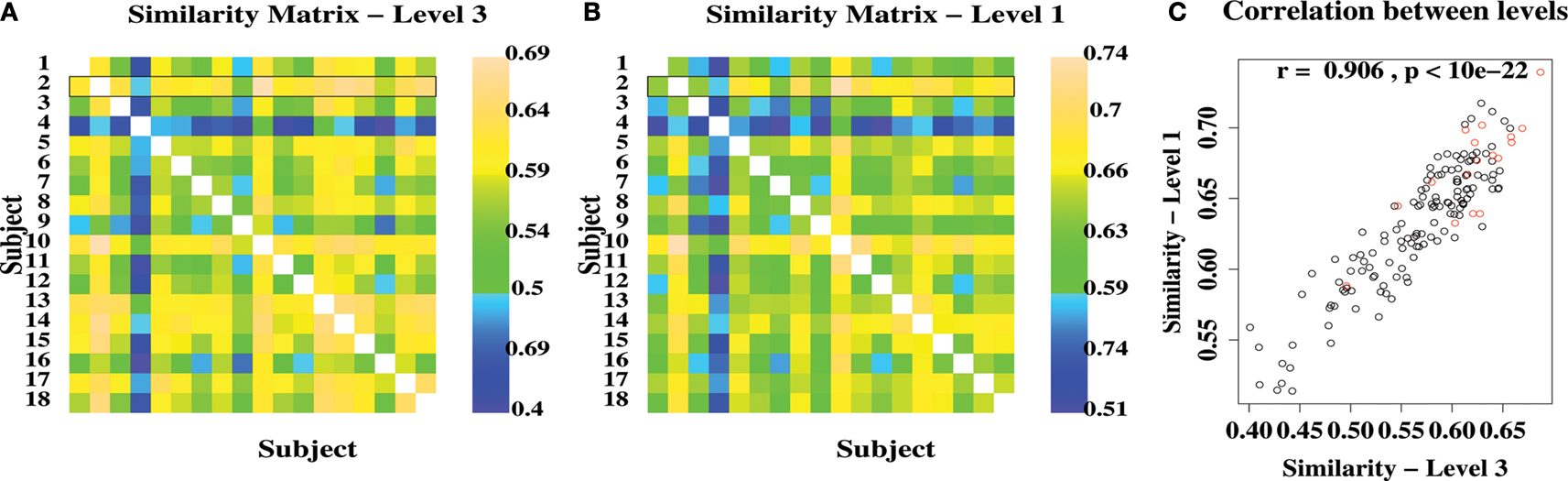
Figure 2. Variability and similarity of brain functional network community structure between 18 different subjects. (A) Matrix showing the between-subject similarity measure for community structure at the highest level of the modular hierarchy. The pairwise similarity scores for the most representative subject are highlighted by a black rectangle. (B) Matrix showing the between-subject similarities for community structure at the lowest level of the modular hierarchy. (C) Scatter plot showing strong correlation of between-subject similarities at high and low levels of the modular hierarchy. Red points are similarities for the most representative subject.
The average pairwise similarity was 0.57 at level 3 and 0.63 at level 1, indicating a reasonable degree of consistency between subjects in modular organization of functional networks. The similarity between subjects was highly correlated over levels of the modular hierarchy: for example, if a pair of networks had a similar modular partition at the highest level, the sub-modular organization at lower levels was also similar.
Simply by summing the pairwise similarity scores for each row of the similarity matrix, it was possible to identify the individual subject (number 2) that was most similar to all other subjects in the sample, i.e. the most representative subject, and the subject (4) that was least similar to the rest of the sample. In what follows, we will focus attention on the modular decomposition of the most representative subject.
Hierarchical Modularity
The hierarchical modular decomposition of the most representative subject’s brain functional network is shown in Figure 3
. At the highest level of the hierarchy (level 3), there were eight large modules, each comprising more than 10 nodes. At the lowest level of the hierarchy (level 1), there were 57 sub-modules. The largest five modules (with putative functional interpretations) and their sub-modular decomposition are briefly described below; some additional details are provided in Table 1
.
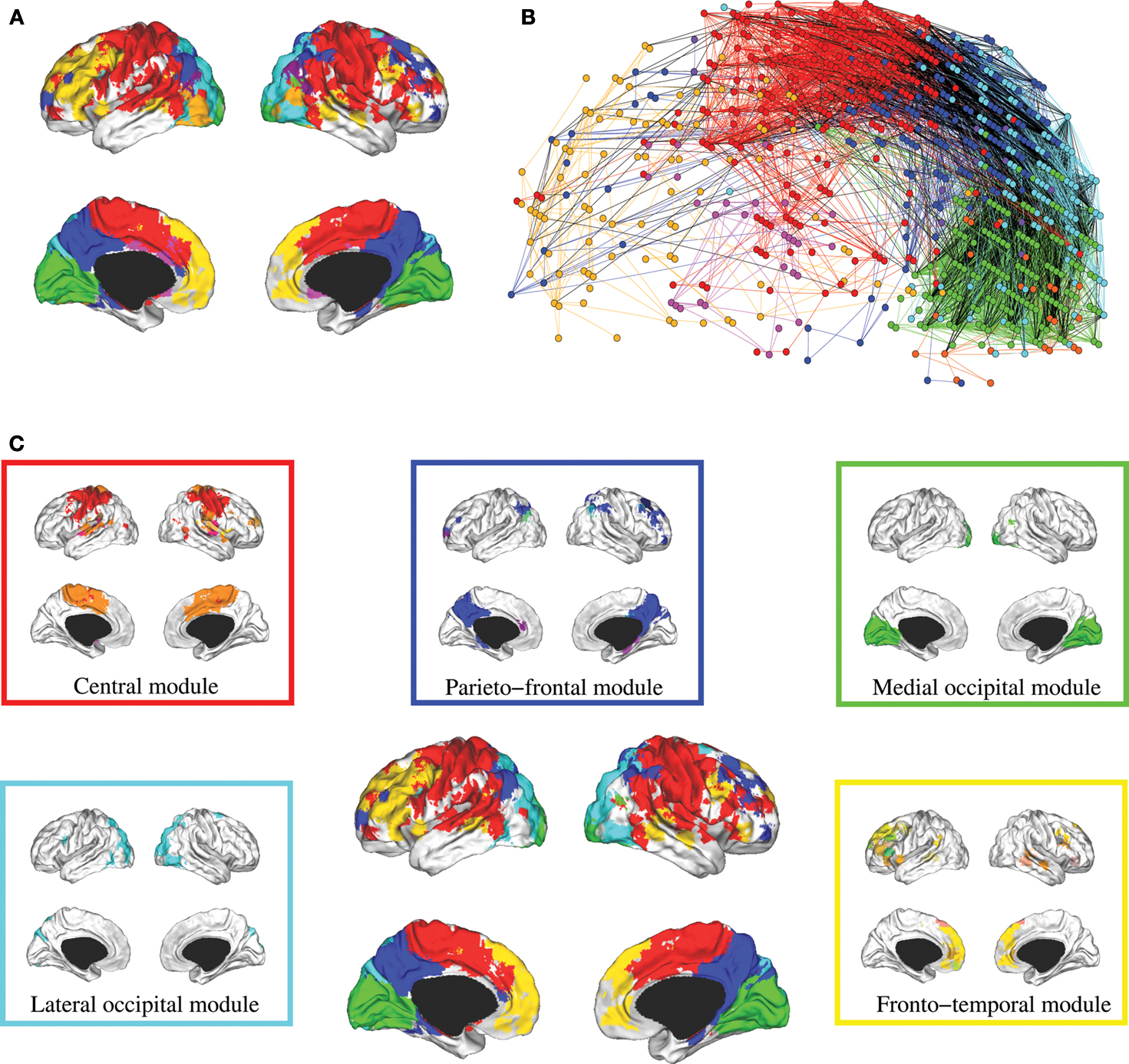
Figure 3. Hierarchical modularity of a human brain functional network. (A) Cortical surface mapping of the community structure of the network at the highest hierarchical level of modularity, showing all modules that comprise more than 10 nodes. (B) Anatomical representation of the connectivity between nodes in colour-coded modules. The brain is viewed from the left side with the frontal cortex on the left of the panel and the occipital cortex on the right of the panel. Intra-modular edges are coloured differently for each module; inter-modular edges are drawn in black. (C) Sub-modular decomposition of the five largest modules (shown centrally) illustrates that the medial occipital module has no major sub-modules whereas the fronto-temporal modules has many sub-modules.
• Central module (somatosensorimotor): The largest high level module comprised extensive areas of lateral cortex in premotor, precentral and postcentral areas, extending inferiorly to superior temporal gyrus, as well as to premotor and dorsal cingulate cortex medially. At a lower hierarchical level, medial and lateral cortex were segregated in different sub-modules and, within lateral cortex, precentral and postcentral areas were segregated from superior temporal cortex.
• Parieto-frontal module (default/attentional): This module comprised medial posterior parietal and posterior cingulate cortex, extending to medial temporal lobe structures inferiorly, and areas of inferior parietal and dorsal prefrontal cortex laterally.
• Medial occipital module (primary visual): This module comprised medial occipital cortex and occipital pole, including primary visual areas.
• Lateral occipital (secondary visual): This module comprised dorsal and ventral areas of lateral occipital cortex, including secondary visual areas.
• Fronto-temporal module (symbolic): This module comprised dorsal and ventral lateral prefrontal cortex, medial prefrontal cortex, and areas of superior temporal cortex. It was less symmetrically organized than most of the other high level modules and was decomposed to a larger number of sub-modules at lower levels.
Note that most high level modules are bilaterally symmetrical, comprise both lateral and medial cortical areas, and tend to be spatially concentrated in an anatomical neighbourhood. Sub-modular decomposition sometimes resulted in a dominant sub-module, comprising most of the nodes in the higher level module, with some much smaller sub-modules each comprising a few peripheral nodes. For example, this was the pattern for the occipital modules. An alternative result was a more even-handed decomposition of a high level module into multiple sub-modules; this was the pattern for the prefronto-temporal module. In Simon’s terminology, the number of sub-modules into which a module can be decomposed is its span of control, and so we can describe occipital modules as having a greater span of control than, say, the fronto-temporal module.
Node Roles
On the basis of the highest level (level 3) of modular decomposition, we assigned topological roles to each of the regional nodes. A node was defined as a hub or non-hub (more or less highly connected) with a provincial, connector or kinless role (depending on its balance of intra- vs inter-module connectivity). Provincial hubs will play a key role in intra-modular processing; connector hubs will play a key role in inter-modular processing.
Figure 4
displays an example of the node roles obtained from the most representative subject. Figure 4
A shows the participation coefficient (P, our measure of inter-modular connectivity) vs the intra-modular degree (z, our measure of hubness) for each regional node in the network. Most nodes (416, 53%) have no inter-modular connections P = 0, but some (28, 4%) have a high proportion of inter-modular connections, qualifying for connector status. Figure 4
B is a spatial representation of the node roles, the locations of the nodes corresponding to their position in three-dimensional stereotactic space. Figure 4
C is a topological representation obtained by applying the Fruchterman–Reingold algorithm (Fruchterman and Reingold, 1991
) to the network displayed in Figure 4
B. In this representation, the distances between the nodes are not related to their spatial location, but to how strongly linked connected they are to their neighbours. The main idea is to start from an initial random placement of the nodes, and replace the edges by springs, letting the equivalent mechanical system evolve until it reaches a stable mechanical state. Thus, this representation locates nodes with similar connectivity patterns closer together in space.
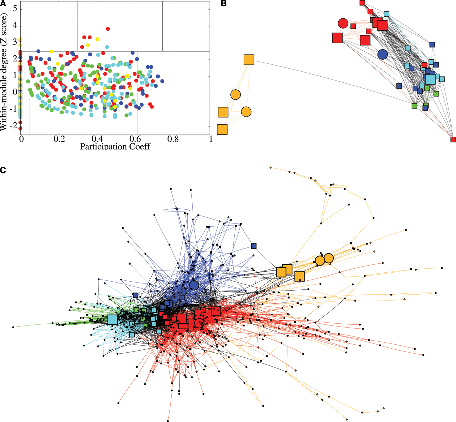
Figure 4. Topological roles of network nodes in intra- and inter-modular connectivity. (A) All nodes are plotted in the {P − z} plane of intra-modular degree z vs participation coefficient P; the solid lines partition the plane according to criteria for hubs vs non-hubs and connector, provincial, peripheral or kinless nodes. (B) Anatomical representation of the provincial hubs (circles), connector hubs (large squares) and connector nodes (small squares) of each of each of the five largest modules at the highest level of the modular hierarchy. (C) Topological representation of the network in using Fruchterman–Reingold algorithm (Fruchterman and Reingold, 1991
) to highlight topological proximity of highly connected nodes; colour and shape of the nodes represent their modular assignment and topological role as above and in Figure 2
.
We can see that most nodes (743, i.e. 95% of the nodes) have either the role of ultra-peripheral nodes or peripheral nodes and a small minority (39, i.e. 5% of the nodes) have the topologically important roles of hubs and/or connector status. Inter-modular connections, and the connector nodes and hubs which mediate them, are most numerous in posterior modules containing regions of association cortex; the fronto-temporal module is sparsely connected to other modules and the medial occipital module also has relatively few connector nodes.
Methodological Issues
This work is a first attempt to uncover the hierarchical organization of brain functional networks and to compare the stability of hierarchical modular decompositions across individuals. There are, however, three possible weaknesses in our analysis that we would like to address in this section.
Validation of the algorithm
A first consideration concerns the choice of the Louvain method (LM) in order to uncover nested modules in the brain networks. LM was first proposed in order to uncover optimal partitions of a graph by maximising modularity. This is a greedy method which is known to be very fast and very precise (Blondel et al., 2008
), albeit less precise than much slower methods such as simulated annealing (SA). It is interesting to note, however, that this lack of precision may be an advantage, in practice, as it may avoid some of the pitfalls of modularity analysis such as its resolution limit (Fortunato and Barthélemy, 2007
). For instance, it has been recently shown that LM performs much better than SA when applied to benchmark networks with unbalanced modules comprising different numbers of nodes (Lancichinetti and Fortunato, 2009
). We therefore believe that there is good evidence that the top level partitions uncovered by LM are valid. The validity of the intermediate hierarchical levels identified by the algorithm is, however, more arguable, as it has not been studied in detail yet. In order to show the validity of these intermediate levels, we need to verify that the method uncovers all the significant partitions present in the network and only those.
To do so, we have tested LM on a benchmark network with known hierarchical structure (Sales-Pardo et al., 2007
); Figure 5
A). This benchmark network is made of 640 nodes with three levels of organization: small modules comprising 10 nodes, medium-size modules comprising 40 nodes and large modules comprising 160 nodes. The cohesiveness of the hierarchy between levels is tuned by a single parameter σ, i.e. the larger the value of σ, the more difficult it is to find the sub-modules. When applied on this benchmark network, the algorithm finds with an excellent precision the first two levels (16 modules and 64 modules), but does not uncover the partition into 4 modules. This result is to be expected because this partition into four modules is sub-optimal in terms of modularity and can therefore not be uncovered by an aggregative method. This shows that the method can at best uncover the partition optimising modularity and finer partitions. In order to uncover coarser partitions, one needs to decrease the resolution of the method, which can be done by following Reichardt and Bornholdt (2006)
, or Sales-Pardo et al. (2007)
, for instance.
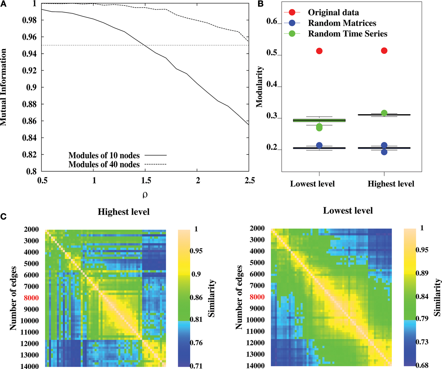
Figure 5. Methodological issues in analysis of hierarchical modularity. (A) Validation of the Louvain method for hierarchical decomposition on a benchmark network defined in Sales-Pardo et al. (2007)
. The network is naturally made of 64, 16 and 4 modules of 10, 40 and 160 nodes respectively. The separability of different levels of the benchmark network is controlled by the parameter ρ. We calculate the normalized information between the lowest non-trivial level partition and the natural partition of 64 modules (solid curve), and between the second level partition and the natural partition of 16 modules (dashed curve). After averaging over 20 different realizations of the network, our simulations show an excellent agreement as mutual information is above 0.95 for values of ρ up to 1.5 for the lowest non-trivial and intermediate levels. (B) Modularity values at the highest and lowest levels of hierarchical community structure in a representative brain network (Subject ID 2, in red) and for networks obtained from 100 randomizations of the original time-series (in green), and for networks obtained by 100 randomizations of the original adjacency matrix. (C) Similarity measures between highest level partitions (left) and non-trivial lowest level partitions (right) obtained by thresholding the original network to retain different number of highest correlations as edges.
On the same benchmark network, the algorithm typically finds two levels (one corresponding to 64 modules and one corresponding to 16 modules) but it may occasionally find three levels (one level corresponding to 64 modules and two levels similar to the partition into 16 modules). When σ = 1.0, for instance, over 100 realizations of the graph, the algorithm finds two levels on 86 realizations, and three levels on 14 realizations. This result is encouraging as it suggests that the algorithm only produces significant partitions. However, it is possible to find situations where it is not the case, e.g. random graphs. It is therefore still necessary to verify the significance of intermediate partitions, as we will discuss below.
Comparison with a random graph
A second consideration concerns the comparison of the partition of the original network with randomized data, as the algorithm also gives a hierarchical decomposition for randomly generated networks. To show that the representative brain network under study (subject ID 2) displays a non-random hierarchical modular structure, we have randomized the original data and processed the hierarchical structure of randomized networks, with two kind of randomization. First, by computing 100 randomizations of the time points in the original time-series (in green on Figure 5
B) and, second, by randomising the original adjacency matrix 100 times (in blue on Figure 5
B). Note that the two kinds of randomization lead to networks with different sizes: in the randomized time-series networks, almost all the nodes are connected, thus leading to networks with 1808 nodes and 8000 edges. Whereas starting from the original adjacency matrix leads to networks of 844 nodes and 8000 edges. The modularity obtained for the lowest and highest partitions of the original network are displayed in Figure 5
B. The modularity values are clearly reduced in the randomized networks, relative to the original data, indicating that our results on real brain networks are not trivially reproduced in random networks.
In order to show that the intermediate levels considered in this paper are significant, we have followed the argument that significant partitions should be robust, in the sense that they should only be weakly altered by a modification of the optimization algorithm. As argued by Ronhovde and Nussinov (2009)
, comparing the optimal partitions found by the algorithm for different orders of the nodes is a way to test their robustness and therefore their validity. We have therefore optimized the modularity of the representative brain network 100 times by choosing the nodes in a different order, and focused on the first non-trivial partition found by the algorithm. The mutual information between pairs of partitions obtained for each different order is then computed. The average mutual information among those pairs is very high (0.89) compared to what is obtained for a comparable random network (0.44), thereby suggesting that partitions obtained at the lowest non-trivial levels are relevant for the network under study.
Dependence on the number of edges
A third consideration concerns the number m of edges that we have chosen in order to map the correlation matrices onto unweighted graphs. This is a known problem when dealing with fMRI data and building brain networks. If m is too small, i.e. keeping the top most significant links, the network will be so sparsely connected that it will be made of several disconnected clusters. If m is too large, in contrast, the network will be very densely connected, but mainly made of unsignificant links. In these two extremes, the network structure is a bad representation of the correlation matrix. This is still an open problem that requires the right trade-off between these two competing factors. In order to show the robustness of our results, we propose to look at the resilience of the hierarchical modular organization under the tuning of the value of m. Meaningful values of m are identified by intervals over which the structure of the network is preserved. We have applied this scheme to the optimal partitions of the most representative subject (Subject 2), over a wide range of threshold (2000–14000 edges, with a step of 200 edges). Our results show that partitions are very similar (in terms of mutual information) over the range (6000–11000) for both highest level (left on Figure 5
C) and non-trivial lowest level (right on Figure 5
C), indicating our results are robust to the specific choice of threshold.
In this study, we have applied recently developed tools for characterizing the hierarchical, modular structure of complex systems to functional brain networks generated from human fMRI data recorded under no-task or resting state conditions. Where previous comparable work was limited by the computational expense of available modularity algorithms, meaning that only one or a few relatively low resolution networks (comprising 10 s of nodes) could be analysed, here we were able to obtain modular decompositions on a larger number of higher resolution networks (each comprising 1000s of nodes). In addition, we used an information-based measure to quantify the similarity of community structure between two different networks and so to find a principled way of focusing attention on a single network that is representative of the group.
Hierarchical Modularity
There was clear evidence for hierarchical modularity in these data and the community structure of the networks at all levels of the hierarchy was reasonably similar across subjects (I ∼ 0.6), suggesting that brain functional modularity is likely to be a replicable phenomenon. This position is further supported by the qualitative similarity between the major modules identified at the highest level of the hierarchy in this study and the major modules or functional clusters identified in comparable prior studies on independent samples (Salvador et al., 2005
; Meunier et al., 2009
). As previously, the major functional modules comprised functionally and/or anatomically related regions of cortex and this pattern was also evident to some extent at sub-modular levels of analysis. For example, the central module comprising areas of somatosensorimotor and premotor cortex was segregated at a sub-modular level into a medial component, comprising supplementary motor area and cingulate motor area, and a lateral component, comprising precentral and postcentral areas of primary motor and somatosensory cortex.
Another plausible aspect of the results was the clear evidence for a symmetrical posterior-to-anterior progression of cortical modules. This was seen most clearly on the medial surfaces of the cerebral hemispheres in terms of their division into medial occipital, parieto-frontal and central modules. A posterior-to-anterior organization of cortical modules in adult brain functional networks is arguably compatible with the abundant evidence from neurodevelopmental studies which have shown rostro-caudal modularity of the spinal cord, brain stem, hind brain and diencephalon defined by segmented patterns of gene expression (Redies and Puelles, 2001
). This speculative link between the topological modularity of adult brain networks and the embryonic modularity of the developing nervous system presents an interesting focus for future studies.
Node Roles in Inter-Modular Connectivity
One important potential benefit of a modular analysis of complex networks is that it allows us to be more precise about the topological role of any particular node in the network. For example, rather than simply saying that a particular region has a high degree we may be able to say that it has a disproportionately important role in transfer of information between modules, rather than within a module. In these data, the location of connector nodes and hubs with a prominent role in inter-modular communication was concentrated in posterior areas of association cortex. The fronto-temporal module, on the other hand, was rather sparsely connected to other modules. One possible explanation for these anatomical differences in inter-modular communication may relate to the stationarity of functional connectivity between brain regions. Our measure of association between brain regions (the wavelet correlation corresponding to a frequency interval of 0.03–0.06 Hz) provides an estimate of functional connectivity “on average” over the entire period of observation (8 min 35 s). If there is significant variability over time in the strength of functional connections between modules this may be manifest in terms of reduced connectivity on average over a prolonged period. Thus one possible explanation for the sparser inter-modular connections of the fronto-temporal module is that the interactions of this system with the rest of the brain network may be more non-stationary or labile over time. This interpretation could be tested by future studies using time-varying measures of functional connectivity, such as phase synchronization (Kitzbichler et al., 2009
).
Dealing with More than One Subject
One of the challenges in analysis of network community structure is the richness of the results (every node will have a modular assignment and a topological role) and the difficulties attendant on properly managing inter-individual variability in such novel metrics. In previous work, we estimated a functional connectivity matrix for each subject, then thresholded the group mean association, and explored the community structure of the group mean network. This allows us to focus attention on a single network but it neglects between-subject variability and, like any use of the mean in small samples, it is potentially biased by one or more outlying values for the functional connectivity. Here we have explored an alternative approach, using an information-based measure of similarity to quantify between subject differences in network organization and to identify the most representative subject in the sample. One can imagine that this measure could be combined with resampling based approaches to statistical inference in order to estimate, for example, the probability that the community structure identified in a single patient is significantly dissimilar to a reference group of brain networks in normal volunteers. However, it fair to say that there are a number of technical challenges to be addressed in using modularity measures for statistical comparisons between different groups.
Returning to Simon’s Hypothesis
As this is the first study to attempt a hierarchical modular decomposition of human brain functional networks, there is little guidance in the existing literature as to what the correct structure of the network should resemble. Our results are encouraging in that they have been able to identify well defined neuroanatomical systems, but they remain empirical and require further validation in appropriate animal models. However, our analysis of simulated data (Section “Discussion”) indicates that our algorithm does indeed identify the correct structure of a hierarchical, modular network, which lends confidence to our results.
In Simon’s theoretical analysis, near-decomposability was considered to be a ubiquitous property of complex systems because it conferred advantages of adaptive speed in response to evolutionary selection pressures as well as shorter-term developmental or environmental contingencies. In relation to the modularity of human brain systems, this view prompts a number of questions. Perhaps the most immediately addressable, at least by functional neuroimaging, is the question of how the modularity of brain network organization relates to cognitive performance and the capacity to shift attention rapidly between different stimuli or tasks. According to Simon’s theory, this key aspect of the brain’s cognitive function should depend critically on modular or sub-modular components and the rapid reconfiguration of inter-modular connections between them. Future studies, applying graph theoretical techniques to modularity analysis of fMRI data recorded during task performance (rather than in no-task state) may be important in testing this prediction.
We have described graph theoretical tools for analysis of hierarchical modularity in human brain functional networks derived from fMRI. Our main claims are that these techniques are computationally feasible and generate plausible and reasonably consistent descriptions of the brain functional network community structure in a group of normal volunteers. The potential importance theoretically of this analysis has been highlighted by reference to Simon’s seminal theory of hierarchy and decomposability in the design of information processing systems.
Edward Bullmore is employed half-time by GlaxoSmithKline and half-time by University of Cambridge.
This research was supported by a Human Brain Project grant from the National Institute of Mental Health and the National Institute of Biomedical Imaging and Bioengineering, National Institutes of Health, Bethesda, MD, USA. Renaud Lambiotte was supported by UK EPSRC. Alex Fornito was supported by a National Health and Medical Research Council CJ Martin Fellowship (ID: 454797). Karen D. Ersche is a recipient of the Betty Behrens Research Fellowship at Clare Hall, University of Cambridge. The experiment was sponsored by GlaxoSmithKline and conducted at the GSK Clinical Unit Cambridge.
Ferrarini, L., Veer, I. M., Baerends, E., van Tol, M.-J., Renken, R. J., Van Der Wee, N. J. A., Veltman, D. J., Aleman, A., Zitman, F. G., Penninx, B. W. J. H., Van Buchem, M. A., Reiber, J. H. C., Rombouts, S. A. R. B., and Milles, J. (2009). Hierarchical functional modularity in the resting-state human brain. Hum. Brain Mapp. 30, 2220–2231.