On the Coherence in the Boundary Layer: Development of a Canopy Interface Model

Introduction

Boundary layer laws have been developed since a very long time. Important characteristics of the surface layer were first described by Prandtl (1925) and these were then recognized as the Prandtl or constant flux layer theories. Subsequently, several studies were conducted to improve the mathematical representation of the different processes taking place in this surface layer and under different atmospheric stability conditions (Monin and Obukhov, 1954; Foken, 2006; Zilitinkevich and Esau, 2007). These theories have been extensively validated with measurements from wind tunnels (Cermak, 1971) as well as measurements in real situations (Businger et al., 1971; Högström, 1990; Beljaars and Holtslag, 1991; Oncley et al., 1996). They are also widely used to calculate the wind profile in specific situations but also to calculate model boundary conditions, for example, in mesoscale meteorological models (Pielke, 2002).

The development of such laws is usually based on the following assumptions (Monin and Obukhov, 1954): (a) it considers meteorological horizontal averages over layers which are long enough to neglect the surface heterogeneity (obstacles are accounted as a roughness that is specified only at the ground level), (b) the size of the eddies generated by the turbulence increases regularly with height, (c) the effect of atmospheric stability is taken into account using specific parameterisations (based on the Richardson number for example). The main disadvantage of these expressions is that they can only be used on restricted situations (e.g., flat surfaces) and as demonstrated by Rotach (1993), Roth (2000), and Karam et al. (2009) they are inappropriate to simulate the flow inside the urban canopy layer. Indeed, in urban areas, complex and heterogeneous obstacles (like buildings) exchange fluxes with all the atmosphere inside the canopy and not only with the ground level as specified in the boundary layer laws. In addition, the presence of obstacles in the canopy disturb the flow in such a way that the assumptions about the eddy sizes (b) and the parameterisation of the atmospheric stability (c) are not valid (Oke, 1987; Foken, 2008). This makes the boundary layer laws unable to simulate accurately the flow inside the urban canopy.

In order to improve the simulation of urban areas in meteorological models, Masson (2000) and other authors (Martilli et al., 2002; Kondo et al., 2005; Masson and Seity, 2009; Krpo et al., 2010; Salamanca et al., 2010) have proposed several 3D parameterisations to calculate fluxes exchanged between the atmosphere and the buildings inside the canopy. None of them computes the modified vertical profiles of meteorological variables inside the urban canopy layer whereas such profiles are crucial for some applications like to estimate accurately heating and cooling energy demands inside buildings (Bueno et al., 2013; Mauree et al., 2015).

The goal of this work is to develop a 1D Canopy Interface Model (CIM) to simulate wind, temperature and turbulent kinetic energy (TKE) profiles inside and above the canopy layer and to use them to calculate of momentum, energy and TKE fluxes. Like for the boundary layer laws, CIM assumes horizontal averages on long layers [assumption (a)]. Based on this assumption, the Navier-Stokes (momentum, heat and TKE) equations are simplified to be discretised and solved only in the vertical direction. On flat surfaces, boundary layer laws (Prandtl, Monin-Obukhov) have been extensively tested and compared against measurements so that they can be considered as reliable references. In this work, we propose a specific formulation and discretisation of the TKE equation to ensure a perfect agreement between the resolution of the simplified Navier-Stokes equations on a flat surface and the Prandtl boundary layer law (neutral stratification). We also propose a correction for the production term of the TKE equation to improve the concordance between the results simulated using the simplified 1D Navier-Stokes equations and the results calculated with the Monin-Obukhov laws (stratified flows). The formulation of the simplified 1D Navier-Stokes equations is then extended to account for heterogeneous obstacles in the airflow. An extension of Santiago and Martilli (2010) formulation for the mixing length is proposed and a discretisation based on Finite Volume Method is implemented to solve the 1D equations. The results calculated with CIM are compared with different kind of results: with the boundary layer laws on flat surfaces (neutral and stratified flows), with results from Large Eddy Simulation (LES) performed over series of obstacles and with experimental data measured during the BUBBLE measurement campaign in Basel (Switzerland). Finally, we look at the implications of this work on the 1D resolution of the Navier-Stokes equation and give a few perspectives.

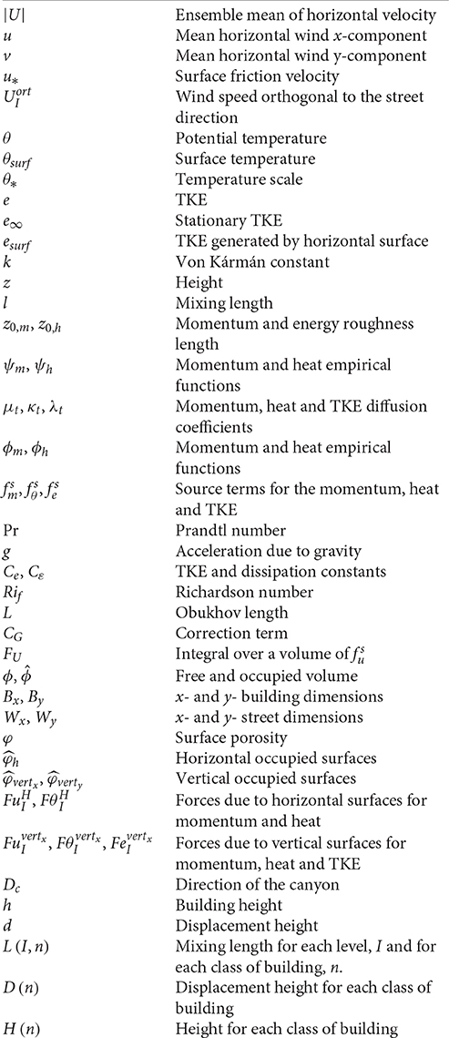
List of Variables

Coherence between Navier-Stokes Resolution and Boundary Layer Laws above a Flat Surface

In the boundary layer, several assumptions can be made. The horizontal wind can be considered to be spatially uniform on average. Furthermore, the friction produced by the surface is simulated as the effect of a roughness that is supposed to represent obstacles randomly dispersed on the ground. The vertical fluxes are constant with height and are equal to the product of vertical gradients of velocity (resp. temperature) and the viscosity (resp. heat conductivity) coefficient. These viscosity and heat conductivity coefficients are written as function of the velocity constant u_* that is proportional to the generated friction and the mixing length that is proportional to the turbulent eddy size. The latter increases with respect to the height. The exchanged fluxes are furthermore modulated by empirical functions (Businger et al., 1971).

Boundary Layer Laws: Monin-Obukhov Equations

For the purpose of this study, we use the Monin-Obukhov analytical solutions. The equations for the wind and temperature are:

$\begin{array}{ll}\left|U\right|=\frac{u_{*}}{k}\left(ln\frac{z}{z_{0,m}}-{\psi }_m\right)and\theta -{\theta }_{surf}=\frac{{\theta }_{*}}{k}\left(ln\frac{z}{z_{0,h}}-{\psi }_h\right),& (1)\end{array}$

where |U| is the ensemble mean of horizontal velocity, θ is the potential temperature, θ_surf is the surface temperature, u_* is the surface friction velocity, θ_* is the temperature scale, k is the von Kármán constant, z is the height and z_{0, m} and z_{0, h} are the momentum and energy roughness length. ψ_m and ψ_h are empirical functions to account for the stability of the atmosphere. More information can be found on them in Jacobson (1999).

In the analytical solution, the momentum (μ_t) and heat (κ_t) diffusion coefficients can be calculated using the following equations:

$\begin{array}{ll}{\mu }_t=\frac{u_{*}kz}{{\varphi }_m}\text{and}{\kappa }_t=\frac{{\theta }_{*}kz}{{\varphi }_h},& (2)\end{array}$

where ϕ_m and ϕ_h are empirical functions first defined by Businger et al. (1971) and later modified by Benoit (1977).

Simplified Navier-Stokes Equations

For a fast resolution of the Navier-Stokes equations in one-dimension, a Canopy Interface Model is developed to resolve meteorological variables over a discretized column. Two assumptions are commonly accepted: the average wind and pressure are horizontally uniform (Holt and Raman, 1988; Stull, 1988; Cuxart et al., 2006).

The differential equations for the momentum and the potential temperature can be written as:

$\begin{array}{ll}\frac{\partial u}{\partial t}=\frac{\partial }{\partial z}\left({\mu }_t\frac{\partial u}{\partial z}\right)+f_m^s\text{and}\frac{\partial \theta }{\partial t}=\frac{\partial }{\partial z}\left({\kappa }_t\frac{\partial \theta }{\partial z}\right)+f_{\theta }^s,& (3)\end{array}$

where u is the mean horizontal wind component in the x- or y-direction, $f_m^s$ and $f_{\theta }^s$ are the terms representing the momentum and heat fluxes exchanged between the flow and “solid” surfaces (ground in our situation). The diffusion coefficients are computed according to a 1.5-order turbulent closure (Equations 7, 8) as proposed by Monin and Yaglom (1971):

$\begin{array}{ll}{\mu }_t=C_e\sqrt{e}l\text{and}{\kappa }_t=\mathrm{Pr}{\mu }_t,& (4)\end{array}$

where C_e is a constant, e is the turbulent kinetic energy (TKE), Pr is the Prandtl number that represents the ratio between the momentum and heat diffusion coefficients, and hence depends on the stability of the atmosphere (Priestley and Swinbank, 1947). In the absence of obstacles, the mixing length, l, is simply given as:

$\begin{array}{ll}l=z\text{.}& (5)\end{array}$

The TKE is calculated, as proposed by Holt and Raman (1988), by using:

$\begin{array}{ll}\frac{\partial e}{\partial t}=\frac{\partial }{\partial z}\left({\lambda }_t\frac{\partial e}{\partial z}\right)+P+G-\epsilon +f_e^s& (6)\end{array}$

$\begin{array}{ll}{\lambda }_t={\mu }_t& (7)\end{array}$

where λ_t is the diffusion coefficient for the TKE. Analogous to the momentum and heat equations, $f_e^s$ represent the additional sources of TKE from the ground. P stands for the mechanical generation of turbulence (due to the shear between air layers). G is the buoyancy term due to temperature difference between each layer. ε represents the TKE dissipation. These three terms can be expressed as follows:

$\begin{array}{ll}P={\mu }_t{\left(\frac{\partial u}{\partial z}\right)}^2; G=\frac{\mathrm{Pr}g}{\theta }{\kappa }_t\left(\frac{\partial \theta }{\partial z}\right);\epsilon =C_{\epsilon }\frac{e^{\frac{3}{2}}}{l},& (8)\end{array}$

where C_ε is a constant.

A Scale for TKE under Neutral Turbulence Condition

In this situation the expected logarithmic solution for the wind speed, above a plane surface, is well known. Similar to Masson and Seity (2009), an analytical solution for TKE can be found using the momentum diffusion coefficient equations (Equations 2, 4) and with ϕ_m = 1 and l = z:

$\begin{array}{ll}{e}_{\infty }={\left(\frac{k{u}_{*}}{C_e}\right)}^2.& (9)\end{array}$

It should be highlighted here that e_∞ is a constant value. In such a case, we propose to write the TKE equation so as to define a stationary value of TKE. Combining Equations (6, 8), as proposed by Holt and Raman (1988), leads to:

$\begin{array}{ll}\frac{\partial e}{\partial t}=\frac{\partial }{\partial z}\left({\lambda }_t\frac{\partial e}{\partial z}\right)+{\mu }_t{\left(\frac{\partial u}{\partial z}\right)}^2-C_{\epsilon }\frac{e^{\frac{3}{2}}}{l} .& (10)\end{array}$

Since the TKE is constant (as demonstrated with Equation 9, over a plane surface), the first two terms of Equation (10) are equal to 0, leading to an equilibrium between production and dissipation:

$\begin{array}{ll}{C}_{\epsilon }\frac{{e_{\infty }}^{\frac{3}{2}}}{l}={\mu }_t{\left(\frac{\partial u}{\partial z}\right)}^2.& (11)\end{array}$

Replacing the diffusion coefficient in the above equation leads to:

$\begin{array}{ll}{C}_{\epsilon }\frac{{e_{\infty }}^{\frac{3}{2}}}{l}=C_e\sqrt{e_{\infty }}l{\left(\frac{\partial u}{\partial z}\right)}^2,& (12)\end{array}$

and the stationary value for the TKE is given by:

$\begin{array}{ll}{e}_{\infty }=\frac{C_e}{C_{\epsilon }}{l}^2{\left(\frac{\partial u}{\partial z}\right)}^2.& (13)\end{array}$

The final TKE equation becomes:

$\begin{array}{ll}\frac{\partial e}{\partial t}=\frac{\partial }{\partial z}\left({\lambda }_t\frac{\partial e}{\partial z}\right)+C_{\epsilon }\frac{\sqrt{e}}{l}\left(e_{\infty }-e\right)+f_e^s.& (14)\end{array}$

As Equations (9, 13) have to give the same result, a relation between the two constants (C_e and C_ε) can be found:

$\begin{array}{ll}\frac{{C_e}^3}{C_{\epsilon }}=k^4& (15)\end{array}$

There is traditionally an inconsistency in the computation of the TKE generated by the ground surfaces, due to the formulation of the TKE equation (Masson and Seity, 2009; Rasheed, 2009). The reason for this is that the TKE is calculated at the center of the cell (as are the other variables such as u) while the ground surface is located at the lower face of the cell. Therefore, the computation of fluxes from the ground are located at the cell face.

The introduction of e_∞, thus solves the numerical problem of the resolution of the TKE equation (see Figure 1). As it was shown that over a plane surface, the TKE is constant, this then implied that both the sources from the horizontal surface, denoted e_surf, and e_∞ are equal. e_∞ can be reformulated using the surface layer, to compute e_surf:

$\begin{array}{ll}{e}_{surf}=\frac{C_e}{C_{\epsilon }}{\left(\frac{u_{*}}{k}\right)}^2,& (16)\end{array}$

thus bringing consistency in the computation of the TKE.

FIGURE 1

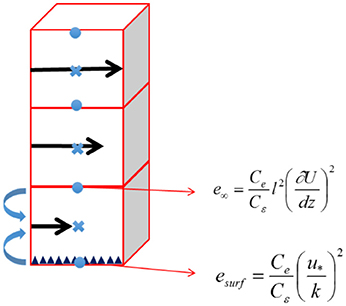
Figure 1. Representation of the new resolution scheme of the TKE in CIM. TKE values can be calculated at the cell's face (dots) and at the center (cross) and then reported at the cell center. Roughness present in the lowest cell of the column.

Stratified Flow

In case of a stratified atmosphere, over a flat surface, the analytical solution given by Equation (9) becomes:

$\begin{array}{ll}e={\left(\frac{k{u}_{*}}{{\varphi }_m{C}_e}\right)}^2.& (17)\end{array}$

This value is not constant anymore with height as ϕ_m is function of z. However, if we want to keep the same formulation as in the neutral case, we can make the following assumption based on the findings from Brouwers (2007) and Charuchittipan and Wilson (2009): locally an equilibrium between the TKE production and dissipation can be observed for any stability cases. Thus, when rewriting with the formulation from the previous section and taking into account the buoyancy from Equation (8), e_∞ becomes:

$\begin{array}{ll}{e}_{\infty }=\frac{C_e}{C_{\epsilon }}{l}^2\left[{\left(\frac{\partial u}{\partial z}\right)}^2+\frac{\mathrm{Pr}g}{\theta }\left(\frac{\partial \theta }{\partial z}\right)\right].& (18)\end{array}$

This can also be written to include the Richardson number as suggested by Cuxart et al. (2006):

$\begin{array}{ll}{e}_{\infty }=\frac{C_e}{C_{\epsilon }}{l}^2{\left(\frac{\partial u}{\partial z}\right)}^2\left(1-R{i}_f\right)\text{ with}R{i}_f=\mathrm{Pr}\frac{g}{\theta }\left(\frac{\partial \theta }{\partial z}\right)/{\left(\frac{\partial u}{\partial z}\right)}^2.& (19)\end{array}$

This equation should yield the same results as the Equation (17). Replacing the ${\left(\frac{\partial u}{dz}\right)}^2$ term using the surface layer laws, a relation between ϕ_m and Ri_f can be found:

$\begin{array}{ll}{\varphi }_m={\left(1-R{i}_f\right)}^{-\frac{1}{4}}.& (20)\end{array}$

It should be highlighted that this relation is relatively close to those proposed by Businger et al. (1971). Indeed, they proposed formulations for ϕ_m depending in the atmospheric conditions. To be coherent with their formulation, the following modification can be brought:

$\begin{array}{ll}{\varphi }_m={\left(1-C_{G}R{i}_f\right)}^{-\frac{1}{4}}.& (21)\end{array}$

where C_G will vary depending on the atmospheric stability and the height above ground. The introduction of C_G can be interpreted as a modification of the Prandtl number ($\mathrm{\text{Pr}}{}^{*}=C_G.\mathrm{\text{Pr}})$.

According to Businger et al. (1971), in an unstable atmosphere:

$\begin{array}{ll}{\varphi }_m={\left(1-{\gamma }_m\frac{z}{L}\right)}^{-\frac{1}{4}},& (22)\end{array}$

and in a stable atmosphere

$\begin{array}{ll}{\varphi }_m=\left(1+{\beta }_m\frac{z}{L}\right),& (23)\end{array}$

where γ_m and β_m are two constant equal to respectively 19.6 and 6, and

$\begin{array}{ll}R{i}_f{\varphi }_m=\frac{z}{L},& (24)\end{array}$

where L is the Obukhov length (Obukhov, 1949).

Thus, in an unstable atmosphere and over a plane surface, if Equations (21, 22) are equal, it is possible to find a relationship for C_G:

$\begin{array}{ll}{\left(1-C_{G}R{i}_f\right)}^{-\frac{1}{4}}={\left(1-{\gamma }_m\frac{z}{L}\right)}^{-\frac{1}{4}},& (25)\end{array}$

$\begin{array}{ll}{\left(1-C_G\frac{z}{L}\frac{1}{{\varphi }_m}\right)}^{-\frac{1}{4}}={\left(1-{\gamma }_m\frac{z}{L}\right)}^{-\frac{1}{4}},& (26)\end{array}$

$\begin{array}{ll}{C}_G={\gamma }_m{\varphi }_m={\gamma }_m{\left(1-{\gamma }_m\frac{z}{L}\right)}^{-\frac{1}{4}}.& (27)\end{array}$

The same reasoning can be applied for the stable case with Equation (21, 23):

$\begin{array}{ll}{\left(1-C_G\frac{z}{L}\frac{1}{{\varphi }_m}\right)}^{-\frac{1}{4}}=\left(1+{\beta }_m\frac{z}{L}\right).& (28)\end{array}$

If |C_GRi_f| ≪ 1 it is possible to eliminate the power functions using the Taylor series:

$\begin{array}{ll}\left(1+C_G\frac{z}{4L}\frac{1}{{\varphi }_m}\right)=\left(1+{\beta }_m\frac{z}{L}\right),& (29)\end{array}$

$\begin{array}{ll}{C}_G=4{\beta }_m{\varphi }_m=4{\beta }_m\left(1+{\beta }_m\frac{z}{L}\right).& (30)\end{array}$

These proposed corrections (Equations 27, 30) bring coherency to the TKE equations w.r.t. the surface layer laws and the governing equation finally becomes:

$\begin{array}{ll}\frac{\partial e}{\partial t}=\frac{\partial }{\partial z}\left({\lambda }_t\frac{\partial e}{\partial z}\right)+C_{\epsilon }\frac{\sqrt{e}}{l}\left(e_{\infty }-e\right)+f_e^s.& (31)\end{array}$

where

$\begin{array}{ll}{e}_{\infty }=\frac{C_e}{C_{\epsilon }}{l}^2{\left(\frac{\partial u}{\partial z}\right)}^2\left[{\left(\frac{\partial u}{\partial z}\right)}^2+C_G\text{Pr}\frac{g}{\theta }\left(\frac{\partial \theta }{\partial z}\right)\right].& (32)\end{array}$

Stevens et al. (1999), who also worked on the development of the turbulence in the boundary layer but in 3D using LES, found a similar formulation for the TKE production: it is a function of a Richardson number multiplied by a correction term C_G which depends on the atmospheric stability. The fact that the Richardson number cannot be calculated when the shear stress is very low, implies that these kind of formulation cannot be applied in the case of free convection.

One can note that, in comparison to the formulation of Stevens et al. (1999), our C_G correction term has been derived for a 1D case and does not need any assumptions on the mixing length. This will give us the freedom to modify it as a function of the obstacle / building density in the canopy layer in next part of the article.

Introduction of Urban Obstacles in the Navier-Stokes Resolution

The formulation derived in Section Coherence between Navier-Stokes Resolution and Boundary Layer Laws above a Flat Surface are developed for a layer above a plane surface. We here extend them for use in an urban roughness layer. As done by Martilli et al. (2002) and others, source terms are added in the $f_u^s{f}_{\theta }^s$ and $f_e^s$ terms of Equations (3, 6), to account for the dynamic and energetic effects of buildings or trees (termed here as urban obstacles). Further propositions are done to take into account varying dimensions.

Discretisation of the Navier-Stokes Equation Using Geometrical Characteristics of the Urban Obstacles

We choose here to discretize Equations (3, 6) by using a finite volume method as it helps to better account for the urban obstacles effects on the air flow. Here for a sake of simplicity, we only show the discretized equation for the momentum in the x−direction. However, the same discretization methodology can be applied for the y−component of the momentum as well as for the discretization of the TKE and heat equations. We propose to determine the solution using:

$\begin{array}{ll}\begin{array}{l}{u}_I^{t+1}=u_I^t+\Delta t\frac{S_i}{V_I}{\mu }_{t_i}\frac{u_{I-1}^t-u_I^t}{\Delta z}-\Delta t\frac{S_{i+1}}{V_I}{\mu }_{t_{i+1}}\frac{u_I^t-u_{I+1}^t}{\Delta z}\\ +\Delta t{F}_u,\end{array}& (33)\end{array}$

where S and V are the surface and volume characteristics of the grid cells respectively, Δz is the height of the grid cell and F_U is the integral over a volume of $f_u^s$ [for additional information please refer to Martilli et al. (2002)]. i and I are indices representing the cell face or center respectively and will be used as such in the following sections of this article.

With immersed obstacles, these grid cell's surfaces and volumes are however reduced modifying the capability of the fluid to exchange meteorological quantities. Until now, obstacles in urban canopy models were only described as arrays of regular cubes uniformly distributed in a grid cell, whose dimensions were uniform with height (Masson, 2000; Martilli et al., 2002). The size of the obstacles can vary for the x- and y-directions at each level of the grid cell in CIM.

Analogous to the definition of the porosity of a material, we define surface and volume porosities as the respective remaining free surface and volume of the grid cells (Krpo et al., 2010). Porosities in contrast to other obstacle morphological indices are a-dimensional and authorize the coupling of CIM with any other urban canopy or building energy models of varying degree of complexity in the urban obstacle geometry representation.

They are computed based on the urban obstacle dimensions. By definition, they vary between 0 and 1, with 1 meaning that the entire surface or volume of the grid cell is free. Figure 2 describes the 3D-geometry of obstacles as well as the resulting surface and volume porosities.

FIGURE 2

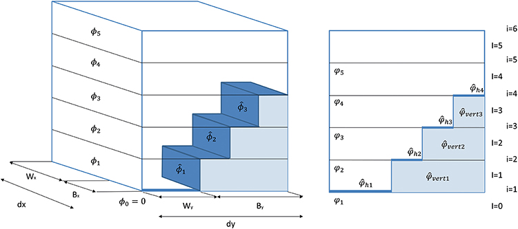
Figure 2. On the left: 3D-view of obstacles with the occupied and free volume (B_x and B_y are the building length and W_x and W_y are the street width in the x- and y-directions respectively. dx and dy are the horizontal grid resolution); on the right: side view of a section of the 1D-column showing the interpretation of the occupied surface and porosities in CIM.

The volume porosity (i.e., the empty volume of the grid cell) is:

$\begin{array}{ll}\varphi (I)=1-\widehat{\varphi }(I),& (34)\end{array}$

where the occupied volume $\widehat{\varphi }$ is given by:

$\begin{array}{ll}\widehat{\varphi }\text{}\left(I\right)=\frac{B_x(I)}{B_x(I)+W_x(I)}\frac{B_y(I)}{B_y(I)+W_y(I)},& (35)\end{array}$

where B_x and B_y are the building lengths and W_x and W_y are the street widths in the x- and y-directions respectively.

Based on volume porosity, the surface porosity (i.e., the empty surface at the grid cells interface) can be calculated as follows:

$\begin{array}{ll}\phi (i)=\text{min}(\varphi \left(I\right),\varphi (I-1)).& (36)\end{array}$

The urban obstacles horizontal (${\widehat{\phi }}_h$) surfaces (as shown in Figure 2) at each level, over the total volume of the grid cell, are computed as:

$\begin{array}{ll}{\widehat{\phi }}_h\text{}\left(i\right)=\frac{\varphi (I)-\varphi (I-1)}{\Delta z}.& (37)\end{array}$

The vertical (${\widehat{\phi }}_{ver{t}_x}$ and ${\widehat{\phi }}_{ver{t}_y}$) surfaces that represent the total occupied surfaces, perpendicular to the x- and y-directions respectively, over the total volume of the grid cell can be found using:

$\begin{array}{ll}{\widehat{\phi }}_{ver{t}_x}\text{}\left(I\right)=\frac{B_x(I)}{B_x(I)+W_x(I)}\frac{B_y(I)}{B_y(I)+W_y(I)}\frac{1}{B_x(I)}& (38)\end{array}$

$\begin{array}{ll}{\widehat{\phi }}_{ver{t}_y}\text{}\left(I\right)=\frac{B_x(I)}{B_x(I)+W_x(I)}\frac{B_y(I)}{B_y(I)+W_y(I)}\frac{1}{B_y(I)}.& (39)\end{array}$

The occupied and free volumes and surfaces are used (1) in the calculations of the diffusion coefficients to represent the reduction of the turbulence exchanges within the urban canopy layer; but also (2) in the formalization of the surface fluxes equations where they are acting as a weighted factor (i.e., the surface fluxes induced by each surface of an urban obstacle are computed according to the corresponding obstacle surface's area).

A representation of the forces induced by the urban obstacles and the different terms can be seen in Figure 3. We slightly modified the formulation proposed by Martilli et al. (2002) to introduce the surface and volume characteristics and present the proposed formulation in Data sheet 1 Annex A: Forces induced by urban obstacles.

FIGURE 3

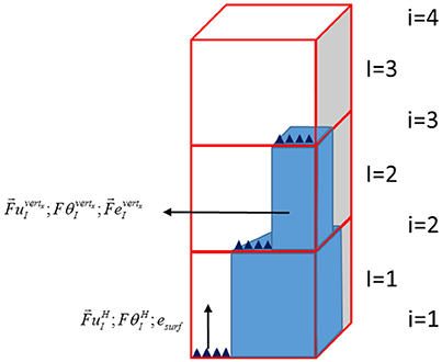
Figure 3. Representation of fluxes from the vertical and horizontal surface when obstacles are integrated in CIM.

Use of the Vertical Distribution of Porosities in the Computation of the Mixing Length

In the presence of urban obstacles, their geometry limits the maximum distance that an air parcel can travel (the maximum free path). To take this into account, Santiago and Martilli (2010) proposed a new formulation. They argued that inside the canopy the mixing length was close to a constant which corresponds to the findings of Raupach et al. (1996).

The mixing length is calculated as:

$\begin{array}{ll}l\text{}\left(i\right)=\text{max}(h-d, z\text{}\left(i\right)-d),& (40)\end{array}$

where h is the obstacle's height, the zero-plane displacement height was defined using:

$\begin{array}{ll}d=h{(1-\varphi )}^{\alpha },& (41)\end{array}$

and ϕ is the volume porosity and α is a constant equal to 0.13.

In the present study, propose to account for the variation of the urban obstacles height within the canopy. The methodology was based on following steps:

1. the buildings were classified according to their height;

2. the ratio of each class in a grid cell was computed;

3. a mixing length for each building class was computed as if this class occupied the whole grid box, and

4. a mean mixing length was calculated based on the ratios of each building class in the grid box.

Figure 4 gives an example, where three classes of buildings were considered with seven buildings present in the grid box. If we consider N classes of buildings with a height (denoted H(n), n = 1, N) which follows the vertical grid (i.e., the top of each grid cell), the ratio of each class can be written using the occupied built volume in the grid as follows:

$\begin{array}{ll}P\left(n\right)=\frac{1}{\widehat{\varphi }(1)}{\displaystyle \sum _{I=1}^N\left(\widehat{\varphi }\left(I\right)-\widehat{\varphi }(I+1)\right),}& (42)\end{array}$

FIGURE 4

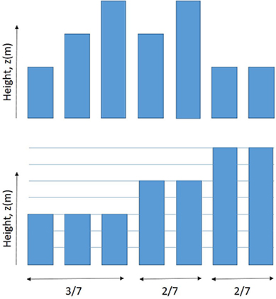
Figure 4. Example of vertical distribution of buildings (top) and their classification in term of height (bottom). N = 3 in this case.

Note that here we assume that the first level is the most occupied level. A weighted mixing length can then be obtained with:

$\begin{array}{ll}l\left(I\right)={\displaystyle \sum _{n=1}^{N}P\left(n\right)L(I,n),}& (43)\end{array}$

where

$\begin{array}{ll}L\text{}\left(I,n\right)=\text{max}\text{}\left(H\left(n\right)-D\text{}\left(n\right),z\text{}\left(I\right)-D\text{}\left(n\right)\right),& (44)\end{array}$

and where the zero-plane displacement height for each building class is:

$\begin{array}{ll}D\text{}\left(n\right)=H\text{}\left(n\right){(1-\varphi (n))}^{\alpha },& (45)\end{array}$

with α still equal to 0.13 like in Santiago and Martilli (2010).

Results and Discussions

CIM Performance under Different Stability Conditions – without Obstacles

Table 1 describes the fixed boundary conditions for the top most cell of CIM for three different atmospheric stability cases defined by means of varying surface temperatures. CIM computations are at this point compared with the analytical solutions given by Equations (1, 9, 17).

TABLE 1

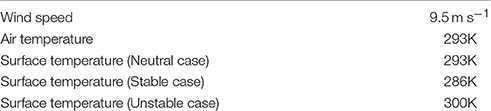
Table 1. Experimental conditions – without obstacles.

Verification of the New Discretization Scheme

To verify the new discretization scheme adopted in CIM, we compare the results obtained in a neutral case with the analytical solution from the surface layer theory.

Figure 5 shows the wind and turbulent kinetic energy profiles. It should be emphasized here that numerical errors due to the new discretization scheme are negligible since there is strictly no difference between the analytical and simulated profiles. This is a significant improvement with regards to other studies which have shown persistent numerical errors in the resolution of the TKE [see for example Masson and Seity (2009) or Rasheed (2009)].

FIGURE 5

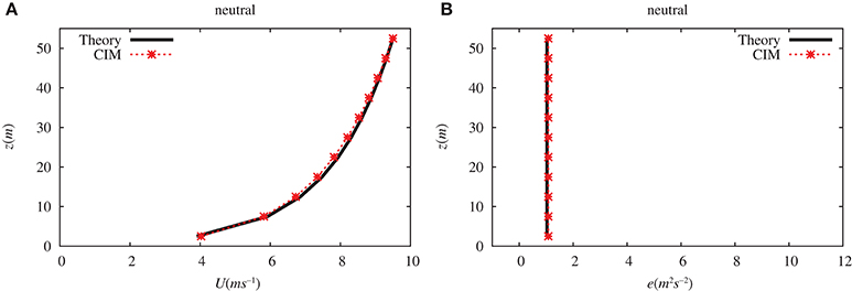
Figure 5. Comparison of (A) the wind (U in m s⁻¹) and (B) the turbulent kinetic energy (e in m² s⁻²) profiles computed over a plane surface using the analytical solution from the surface-layer theory and from CIM under neutral conditions. Altitude (z) is in meters.

Stable and Unstable Case

When considering stable and unstable atmospheric conditions, we also compare the simulation from CIM with the analytical solutions derived from surface layer theory.

Figures 6, 7 give the various profiles for the wind speed, potential temperature and the turbulent kinetic energy. Two different profiles are calculated from CIM – one without and one with the C_G term.

FIGURE 6

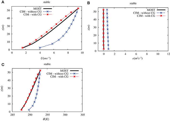
Figure 6. Comparison of (A) the wind (U in m s⁻¹), (B) the turbulent kinetic energy (e in m²s⁻²) and (C) the potential temperature (θ in K) vertical profiles obtained over a plane surface with the surface layer theory and with CIM under stable conditions (with and without the C_G correction). Altitude (z) is in meters.

FIGURE 7

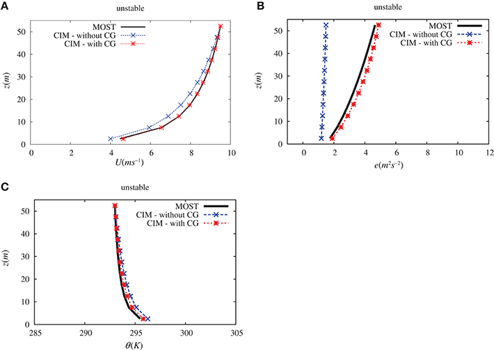
Figure 7. Comparison of (A) the wind (U in m s⁻¹), (B) the turbulent kinetic energy (e in m²s⁻²) and (C) the potential temperature (θ in K) vertical profiles obtained over a plane surface with the surface layer theory and with CIM under unstable conditions (with and without the C_G correction). Altitude (z) is in meters.

It can be highlighted that without the C_G term in the TKE equation, the analytical solution is considerably different from the profiles computed by CIM. On the one hand, in the stable case (see Figure 6), the calculated wind speed is substantially higher as is the potential temperature. The apparent reason for this is that there is an over-estimation of the turbulent kinetic energy and this then leads to an enhance mixing above the surface. On the other hand, with an unstable case (see Figure 7), there is a significant reduction in the turbulent kinetic energy. In this case, however, the reduction in the wind speed and in the temperature is not of the same order of magnitude as the turbulent kinetic energy.

The use of the C_G term in the turbulent kinetic energy noticeably modifies the profiles calculated by CIM. This additional term is necessary to take into account that the fact that the ratio between the diffusion coefficients, usually approximated with the Prandtl number, is not a constant. It thus brings consistency between the traditional formulation of the Navier-Stokes equation and the surface layer theory.

CIM Performance with Urban Obstacles – under Neutral Conditions

To assess CIM's ability to reproduce vertical wind profile in an urban environment, we compare the profile obtained from CIM with those from an LES experiment designed for a regular arrays of cubes (Coceal et al., 2007; Xie et al., 2008) (see Table 2) and with data from the BUBBLE experiment (Rotach et al., 2005; Christen et al., 2009) (see Table 3).

TABLE 2

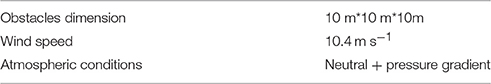
Table 2. LES experimental conditions.

TABLE 3

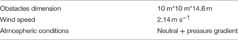
Table 3. BUBBLE experimental conditions.

Comparison with an LES

A comparison of the profiles from the LES and CIM is given in Figure 8. It can be underlined here that the horizontal wind speeds are in very good agreement with each other. Note that there is negative gradient for the TKE above the urban obstacles which reflects the use of a pressure gradient. Although, CIM slightly underestimates the magnitude of the overall TKE, the trend including the height at which the maximum TKE is obtained are in very good accordance with the data from the LES.

FIGURE 8

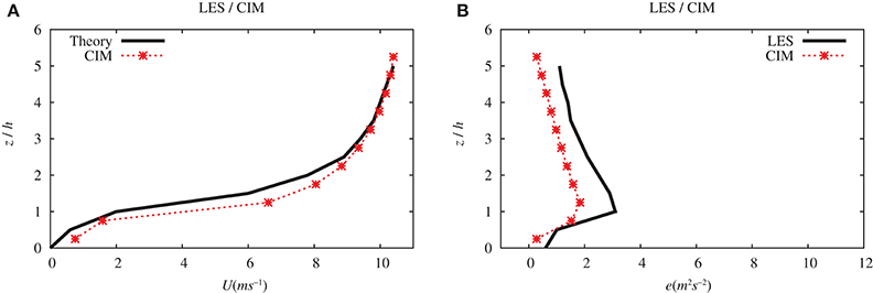
Figure 8. Comparison with data from an LES experiment of the (A) the horizontal wind speed (U in m s⁻¹) and (B) the turbulent kinetic energy (e in m² s⁻²) profiles computed by CIM. Altitude (z) is normalized with the building height.

Comparison with Experimental Data from Bubble

It can be observed from Figure 9 that in general CIM can reproduce the expected profiles. CIM marginally overestimated the wind speed in the urban canyon. One of the reason might be the parameterization of the drag force coefficient that causes a higher wind speed close to ground. Nevertheless, it can be noticed that above the canopy layer, the wind speed computed by CIM is in very good agreement with the measured data.

FIGURE 9

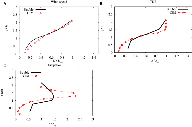
Figure 9. Comparison with data from the Bubble experiment of the (A) horizontal wind speed U (B) the turbulent kinetic energy and (C) dissipation ε, profiles computed by CIM. Variables are normalized by valued at the top of the column and altitude (z) is normalized with the average building height.

Figure 9B shows some differences between the TKE simulated by the CIM model and the data from the Bubble experiment. The overall trend coincides well with the measured data although there are some discrepancies in the magnitude of the maximum TKE budget near the building roofs. This also reflects a similar finding to Santiago and Martilli (2010). For the dissipation term (ε), there is a significant over-estimation from the CIM computation at the roof level (see Figure 9C). Inside the canopy and above the roof the simulation is however in accordance with the measured data. Nevertheless, it can be pointed out that this is a normalized term and when looking at the budget (see Figure 9B), it can be noticed that the difference becomes much smaller between the computed and the experimental data.

Conclusions

In order to develop a coherent resolution of the Navier-Stokes equation in an urban roughness layer, a comparison between the Navier-Stokes resolution and the boundary layer laws was first undertaken. Three essential points have been addressed in this article: the discretization of the TKE, the calculation of the Richardson term in the TKE equation and the extension of the mixing length formulation in an urban canopy with varying dimensions of the buildings.

We proposed a new formulation that brought concordance in the resolution of the TKE equation. First, we demonstrated that in a neutral case and without obstacle, a constant TKE profile should be obtained. Based on this we extended and generalized the equation so that when obstacles are integrated in the canopy, there is no conflict in the computation of the TKE at the face or at the center of the cell.

Additionally, a modification of the Richardson term in the TKE was proposed. This additional term is needed, at least, due to the fact that the Prandtl number is usually considered as a constant. Although this correction brought coherence with the analytical solution, few questions remain regarding the validity of this term beyond the surface layer, especially inside the canopy and in all stability cases. Furthermore, this modification proposed can also be implemented in a 3D RANS model and this could be a possibility for further validation.

Santiago and Martilli (2010) made a proposition for the mixing length in an urban canopy. In this article, we have presented one key adaptation to extend this formulation in case of obstacles with varying heights.

Finally, we validated our model with data from two different experiments: an LES study from Coceal et al., (2007) and with data from the Bubble experiment (Rotach et al., 2005; Christen et al., 2009). Although, there were some discrepancies in the wind speed close to the ground, the simulation results were in very good agreement with the measured data, especially when taking into account the computational time and the fact that CIM is a 1D column module resolving the flow in 2 directions only. Such a module is expected to bridge the gap between meso-scale and micro-scale models by improving the surface representation effect on meteorological variables.

The validation of the Canopy Interface Model needs to be done more extensively specially for stratified flows. However, with the current lack of finding measurements in control environments to compare with the modeling results, it is quite difficult to go beyond the current assessments. Future measurement campaign or wind tunnel experiments could be used for such validation.

Author Contributions

All authors contributed to drafting and revision of the article. DM conducted the experiments and wrote the paper. MK designed and implemented the porosity in the module. NB and AC supervised the experiments and gave advice on the article.

Conflict of Interest Statement

The authors declare that the research was conducted in the absence of any commercial or financial relationships that could be construed as a potential conflict of interest.

Acknowledgments

The authors would like to thank the Agence de la Maîtrise de l'Energie et de l'Environnement, the Region Alsace, REALISE and the Zone Atelier Urbaine Environmentale for the fundings. The research was also performed in the framework of the SCCER Future Energy Efficient Buildings and Districts, FEEB&D, (CTI.2014.0119), ANR Trame Verte, the CCTV2 project. The authors would also like to thank A. Christen for the data from the BUBBLE experiment, Alberto Martilli for the discussions and the reviewers for their comments.

Supplementary Material

The Supplementary Material for this article can be found online at: https://www.frontiersin.org/article/10.3389/feart.2016.00109/full#supplementary-material

Abbreviations

1D, One dimension; CIM, Canopy Interface Model; TKE, Turbulent Kinetic Energy; LES, Large Eddy Simulation.

References

Aumond, P., Masson, V., Lac, C., Gauvreau, B., Dupont, S., and Berengier, M. (2013). Including the drag effects of canopies: real case large-eddy simulation studies. Boundary Layer Meteorol. 146, 65–80. doi: 10.1007/s10546-012-9758-x

CrossRef Full Text | Google Scholar

Beljaars, A., and Holtslag, A. (1991). Flux parameterization over land surfaces for atmospheric models. J. Appl. Meteorol. 30, 327–341. doi: 10.1175/1520-0450(1991)030<0327:FPOLSF>2.0.CO;2

CrossRef Full Text | Google Scholar

Benoit, R. (1977). On the integral of the surface layer profile-gradient functions. J. Appl. Meteorol. 16, 859–860. doi: 10.1175/1520-0450(1977)016<0859:OTIOTS>2.0.CO;2

CrossRef Full Text | Google Scholar

Brouwers, J. J. H. (2007). Dissipation equals production in the log layer of wall-induced turbulence. Phys. Fluids 19:101702. doi: 10.1063/1.2793147

CrossRef Full Text | Google Scholar

Bueno, B., Hidalgo, J., Pigeon, G., Norford, L., and Masson, V. (2013). Calculation of air temperatures above the urban canopy layer from measurements at a rural operational weather station. J. Appl. Meteorol. Climatol. 52, 472–483. doi: 10.1175/JAMC-D-12-083.1

CrossRef Full Text | Google Scholar

Businger, J. A., Wyngaard, J., Izumi, Y., and Bradley, E. F. (1971). Flux-profile relationships in the atmospheric surface layer. J. Atmos. Sci. 28, 181–189. doi: 10.1175/1520-0469(1971)028<0181:FPRITA>2.0.CO;2

CrossRef Full Text | Google Scholar

Cermak, J. E. (1971). Laboratory simulation of the atmospheric boundary layer. AIAA J. 9, 1746–1754. doi: 10.2514/3.49977

CrossRef Full Text | Google Scholar

Charuchittipan, D., and Wilson, J. D. (2009). Turbulent kinetic energy dissipation in the surface layer. Boundary Layer Meteorol. 132, 193–204. doi: 10.1007/s10546-009-9399-x

CrossRef Full Text | Google Scholar

Christen, A., Rotach, M. W., and Vogt, R. (2009). The budget of turbulent kinetic energy in the urban roughness sublayer. Boundary Layer Meteorol. 131, 193–222. doi: 10.1007/s10546-009-9359-5

CrossRef Full Text | Google Scholar

Coceal, O., Dobre, A., Thomas, T. G., and Belcher, S. E. (2007). Structure of turbulent flow over regular arrays of cubical roughness. J. Fluid Mech. 589, 375–409. doi: 10.1017/S002211200700794X

CrossRef Full Text | Google Scholar

Cuxart, J., Holtslag, A. A. M., Beare, R. J., Bazile, E., Beljaars, A., Cheng, A., et al. (2006). Single-column model intercomparison for a stably stratified atmospheric boundary layer. Boundary Layer Meteorol. 118, 273–303. doi: 10.1007/s10546-005-3780-1

CrossRef Full Text | Google Scholar

Foken, T. (2006). 50 years of the monin–obukhov similarity theory. Boundary Layer Meteorol. 119, 431–447. doi: 10.1007/s10546-006-9048-6

CrossRef Full Text | Google Scholar

Foken, T. (2008). Micrometeorology. Berlin: Springer.

Google Scholar

Hamdi, R., and Masson, V. (2008). Inclusion of a drag approach in the Town Energy Balance (TEB) scheme: offline 1D evaluation in a street canyon. J. Appl. Meteorol. Climatol. 47, 2627–2644. doi: 10.1175/2008JAMC1865.1

CrossRef Full Text | Google Scholar

Högström, U. (1990). Analysis of turbulence structure in the surface layer with a modified similarity formulation for near neutral conditions. J. Atmos. Sci. 47, 1949–1972. doi: 10.1175/1520-0469(1990)047<1949:AOTSIT>2.0.CO;2

CrossRef Full Text | Google Scholar

Holt, T., and Raman, S. (1988). A review and comparative evaluation of multilevel boundary layer parameterizations for first-order and turbulent kinetic energy closure schemes. Rev. Geophys. 26, 761–780. doi: 10.1029/RG026i004p00761

CrossRef Full Text | Google Scholar

Jacobson, M. Z. (1999). Fundamentals of Atmospheric Modeling. Cambridge; New York, NY: Cambridge University Press.

Google Scholar

Karam, H. A., Filho, A. J. P., Masson, V., Noilhan, J., and Filho, E. P. M. (2009). Formulation of a tropical town energy budget (t-TEB) scheme. Theor. Appl. Climatol. 101, 109–120. doi: 10.1007/s00704-009-0206-x

CrossRef Full Text | Google Scholar

Kondo, H., Genchi, Y., Kikegawa, Y., Ohashi, Y., Yoshikado, H., and Komiyama, H. (2005). Development of a multi-layer urban canopy model for the analysis of energy consumption in a big city: structure of the urban canopy model and its basic performance. Boundary-Layer Meteorol. 116, 395–421. doi: 10.1007/s10546-005-0905-5

CrossRef Full Text | Google Scholar

Krpo, A., Salamanca, F., Martilli, A., and Clappier, A. (2010). On the impact of anthropogenic heat fluxes on the urban boundary layer: a two-dimensional numerical study. Boundary Layer Meteorol. 136, 105–127. doi: 10.1007/s10546-010-9491-2

CrossRef Full Text | Google Scholar

Louis, J.-F. (1979). A parametric model of vertical eddy fluxes in the atmosphere. Boundary Layer Meteorol. 17, 187–202. doi: 10.1007/BF00117978

CrossRef Full Text | Google Scholar

Martilli, A., Clappier, A., and Rotach, M. W. (2002). An urban surface exchange parameterisation for mesoscale models. Boundary Layer Meteorol. 104, 261–304. doi: 10.1023/A:1016099921195

CrossRef Full Text | Google Scholar

Masson, V. (2000). A physically-based scheme for the urban energy budget in atmospheric models. Boundary Layer Meteorol. 94, 357–397. doi: 10.1023/A:1002463829265

CrossRef Full Text | Google Scholar

Masson, V., and Seity, Y. (2009). Including atmospheric layers in vegetation and urban offline surface schemes. J. Appl. Meteorol. Climatol. 48, 1377–1397. doi: 10.1175/2009JAMC1866.1

CrossRef Full Text | Google Scholar

Mauree, D., Kämpf, J. H., and Scartezzini, J.-L. (2015). “Multi-scale modelling to improve climate data for building energy models,” in Proceedings of the 14th International Conference of the International Building Performance Simulation Association (Hyderabad). Available online at: http://infoscience.epfl.ch/record/214837 (Accessed January 14, 2016).

McAdams, W. (1985). Heat Transmission. New York, NY: McGraw Hill, 1954.

Google Scholar

Mirsadeghi, M., Cóstola, D., Blocken, B., and Hensen, J. L. M. (2013). Review of external convective heat transfer coefficient models in building energy simulation programs: implementation and uncertainty. Appl. Therm. Eng. 56, 134–151. doi: 10.1016/j.applthermaleng.2013.03.003

CrossRef Full Text | Google Scholar

Monin, A. S., and Obukhov, A. M. (1954). Basic laws of turbulent mixing in the surface layer of the atmosphere. Contrib. Geophys. Inst. Acad. Sci. USSR 151, 163–187.

Google Scholar

Monin, A., and Yaglom, A. (1971). Statistical Fluid Dynamics, Vol. 1, 2. Cambridge: MIT Press.

Obukhov, A. (1949). Temperature field structure in a turbulent flow. Izv. Acad. Nauk SSSR Ser. Geog. Geofiz 13, 58–69.

Oke, T. (1987). Boundary Layer Climates. London: Methuen and Co., Ltd.

Google Scholar

Oncley, S. P., Friehe, C. A., Larue, J. C., Businger, J. A., Itsweire, E. C., and Chang, S. S. (1996). Surface-layer fluxes, profiles, and turbulence measurements over uniform terrain under near-neutral conditions. J. Atmos. Sci. 53, 1029–1044. doi: 10.1175/1520-0469(1996)0531029:SLFPAT>2.0.CO;2

CrossRef Full Text | Google Scholar

Otte, T. L., Lacser, A., Dupont, S., and Ching, J. K. S. (2004). Implementation of an urban canopy parameterization in a mesoscale meteorological model. J. Appl. Meteorol. 43, 1648–1665. doi: 10.1175/JAM2164.1

CrossRef Full Text | Google Scholar

Pielke, R. A. (2002). Mesoscale Meteorological Modeling. San Diego, CA: Academic press.

Google Scholar

Prandtl, L. (1925). Report on Investigation of Developed Turbulence. NACA Report TM-1231.

Priestley, C. H. B., and Swinbank, W. C. (1947). Vertical transport of heat by turbulence in the atmosphere. Proc. R. Soc. Lond. Ser. A 189, 543–561. doi: 10.1098/rspa.1947.0057

CrossRef Full Text | Google Scholar

Rasheed, A. (2009). Multiscale Modelling of Urban Climate. Ph.D. thesis, EPFL #4531.

Raupach, M. R. (1992). Drag and drag partition on rough surfaces. Boundary Layer Meteorol. 60, 375–395. doi: 10.1007/BF00155203

CrossRef Full Text | Google Scholar

Raupach, M. R., Finnigan, J. J., and Brunei, Y. (1996). Coherent eddies and turbulence in vegetation canopies: the mixing-layer analogy. Boundary Layer Meteorol. 78, 351–382. doi: 10.1007/BF00120941

CrossRef Full Text | Google Scholar

Rotach, M. W. (1993). Turbulence close to a rough urban surface part I: reynolds stress. Boundary Layer Meteorol. 65, 1–28. doi: 10.1007/BF00708816

CrossRef Full Text | Google Scholar

Rotach, M. W., Vogt, R., Bernhofer, C., Batchvarova, E., Christen, A., Clappier, A., et al. (2005). BUBBLE – an urban boundary layer meteorology project. Theor. Appl. Climatol. 81, 231–261. doi: 10.1007/s00704-004-0117-9

CrossRef Full Text | Google Scholar

Roth, M. (2000). Review of atmospheric turbulence over cities. Q. J. R. Meteorol. Soc. 126, 941–990. doi: 10.1002/qj.49712656409

CrossRef Full Text | Google Scholar

Salamanca, F., Krpo, A., Martilli, A., and Clappier, A. (2010). A new building energy model coupled with an urban canopy parameterization for urban climate simulations—part I. formulation, verification, and sensitivity analysis of the model. Theor. Appl. Climatol. 99, 331–344. doi: 10.1007/s00704-009-0142-9

CrossRef Full Text | Google Scholar

Santiago, J. L., Coceal, O., Martilli, A., and Belcher, S. E. (2008). Variation of the sectional drag coefficient of a group of buildings with packing density. Boundary Layer Meteorol. 128, 445–457. doi: 10.1007/s10546-008-9294-x

CrossRef Full Text | Google Scholar

Santiago, J. L., and Martilli, A. (2010). A dynamic urban canopy parameterization for mesoscale models based on computational fluid dynamics reynolds-averaged navier–stokes microscale simulations. Boundary Layer Meteorol. 137, 417–439. doi: 10.1007/s10546-010-9538-4

CrossRef Full Text | Google Scholar

Stevens, B., Moeng, C.-H., and Sullivan, P. P. (1999). Large-eddy simulations of radiatively driven convection: sensitivities to the representation of small scales. J. Atmos. Sci. 56, 3963–3984. doi: 10.1175/1520-0469(1999)056<3963:LESORD>2.0.CO;2

CrossRef Full Text | Google Scholar

Stull, R. B. (1988). An Introduction to Boundary Layer Meteorology. Dordrecht: Kuler Academic Publishers.

Google Scholar

Xie, Z.-T., Coceal, O., and Castro, I. P. (2008). Large-eddy simulation of flows over random urban-like obstacles. Boundary Layer Meteorol. 129:1. doi: 10.1007/s10546-008-9290-1

CrossRef Full Text | Google Scholar

Zilitinkevich, S., and Esau, I. (2007). Similarity theory and calculation of turbulent fluxes at the surface for the stably stratified atmospheric boundary layer. Boundary Layer Meteorol. 125, 193–205. doi: 10.1007/s10546-007-9187-4

CrossRef Full Text | Google Scholar