JIDT: an information-theoretic toolkit for studying the dynamics of complex systems

1. Introduction

Information theory was originally introduced by Shannon (1948) to quantify fundamental limits on signal processing operations and reliable communication of data (Cover and Thomas, 1991; MacKay, 2003). More recently, it is increasingly being utilized for the design and analysis of complex self-organized systems (Prokopenko et al., 2009). Complex systems science (Mitchell, 2009) is the study of large collections of entities (of some type), where the global system behavior is a non-trivial result of the local interactions of the individuals, e.g., emergent consciousness from neurons, emergent cell behavior from gene regulatory networks and flocks determining their collective heading. The application of information theory to complex systems can be traced to the increasingly popular perspective that commonalities between complex systems may be found “in the way they handle information” (Gell-Mann, 1994). Certainly, there have been many interesting insights gained from the application of traditional information-theoretic measures such as entropy and mutual information to study complex systems, for example, proposals of candidate complexity measures (Tononi et al., 1994; Adami, 2002), characterizing order-chaos phase transitions (Miramontes, 1995; Solé and Valverde, 2001; Prokopenko et al., 2005, 2011), and measures of network structure (Solé and Valverde, 2004; Piraveenan et al., 2009).

More specifically though, researchers are increasingly viewing the global behavior of complex systems as emerging from the distributed information processing, or distributed computation, between the individual elements of the system (Langton, 1990; Mitchell, 1998; Fernández and Solé, 2006; Wang et al., 2012; Lizier, 2013), e.g., collective information processing by neurons (Gong and van Leeuwen, 2009). Computation in complex systems is examined in terms of: how information is transferred in the interaction between elements, how it is stored by elements, and how these information sources are non-trivially combined. We refer to the study of these operations of information storage, transfer, and modification, and in particular, how they unfold in space and time, as information dynamics (Lizier, 2013; Lizier et al., 2014).

Information theory is the natural domain to quantify these operations of information processing, and we have seen a number of measures recently introduced for this purpose, including the well-known transfer entropy (Schreiber, 2000), as well as active information storage (Lizier et al., 2012b) and predictive information (Bialek et al., 2001; Crutchfield and Feldman, 2003). Natural affinity aside, information theory offers several distinct advantages as a measure of information processing in dynamics¹, including its model-free nature (requiring only access to probability distributions of the dynamics), ability to handle stochastic dynamics, and capture non-linear relationships, its abstract nature, generality, and mathematical soundness.

In particular, this type of information-theoretic analysis has gained a strong following in computational neuroscience, where the transfer entropy has been widely applied (Honey et al., 2007; Vakorin et al., 2009; Faes et al., 2011; Ito et al., 2011; Liao et al., 2011; Lizier et al., 2011a; Vicente et al., 2011; Marinazzo et al., 2012; Stetter et al., 2012; Stramaglia et al., 2012; Mäki-Marttunen et al., 2013; Wibral et al., 2014b,c) (for example, for effective network inference), and measures of information storage are gaining traction (Faes and Porta, 2014; Gómez et al., 2014; Wibral et al., 2014a). Similarly, such information-theoretic analysis is popular in studies of canonical complex systems (Lizier et al., 2008c, 2010, 2012b; Mahoney et al., 2011; Wang et al., 2012; Barnett et al., 2013), dynamics of complex networks (Lizier et al., 2008b, 2011c, 2012a; Damiani et al., 2010; Damiani and Lecca, 2011; Sandoval, 2014), social media (Bauer et al., 2013; Oka and Ikegami, 2013; Steeg and Galstyan, 2013), and in artificial life and modular robotics both for analysis (Lungarella and Sporns, 2006; Prokopenko et al., 2006b; Williams and Beer, 2010a; Lizier et al., 2011b; Boedecker et al., 2012; Nakajima et al., 2012; Walker et al., 2012; Nakajima and Haruna, 2013; Obst et al., 2013; Cliff et al., 2014) and design (Prokopenko et al., 2006a; Ay et al., 2008; Klyubin et al., 2008; Lizier et al., 2008a; Obst et al., 2010; Dasgupta et al., 2013) of embodied cognitive systems (in particular, see the “Guided Self-Organization” series of workshops, e.g., (Prokopenko, 2009)).

This paper introduces JIDT – the Java Information Dynamics Toolkit – which provides a standalone implementation of information-theoretic measures of dynamics of complex systems. JIDT is open-source, licensed under GNU General Public License v3, and available for download via Google code at http://code.google.com/p/information-dynamics-toolkit/. JIDT is designed to facilitate general-purpose empirical estimation of information-theoretic measures from time-series data, by providing easy to use, portable implementations of measures of information transfer, storage, shared information, and entropy.

We begin by describing the various information-theoretic measures, which are implemented in JIDT in Section 2.1 and Section S.1 in Supplementary Material, including the basic entropy and (conditional) mutual information (Cover and Thomas, 1991; MacKay, 2003), as well as the active information storage (Lizier et al., 2012b), the transfer entropy (Schreiber, 2000), and its conditional/multivariate forms (Lizier et al., 2008c, 2010). We also describe how one can compute local or pointwise values of these information-theoretic measures at specific observations of time-series processes, so as to construct their dynamics in time. We continue to then describe the various estimator types, which are implemented for each of these measures in Section 2.2 and Section S.2 in Supplementary Material (i.e., for discrete or binned data, and Gaussian, box-kernel, and Kraskov–Stögbauer–Grassberger estimators). Readers familiar with these measures and their estimation may wish to skip these sections. We also summarize the capabilities of similar information-theoretic toolkits in Section 2.3 (focusing on those implementing the transfer entropy).

We then turn our attention to providing a detailed introduction of JIDT in Section 3, focusing on the current version 1.0 distribution. We begin by highlighting the unique features of JIDT in comparison to related toolkits, in particular, in providing local information-theoretic measurements of dynamics; implementing conditional, and other multivariate transfer entropy measures; and including implementations of other related measures including the active information storage. We describe the (almost 0) installation process for JIDT in Section 3.1: JIDT is standalone software, requiring no prior installation of other software (except a Java Virtual Machine), and no explicit compiling or building. We describe the contents of the JIDT distribution in Section 3.2, and then in Section 3.3 outline, which estimators are implemented for each information-theoretic measure. We then describe the principles behind the design of the toolkit in Section 3.4, including our object-oriented approach in defining interfaces for each measure, then providing multiple implementations (one for each estimator type). Sections 3.5 and 3.7 then describe how the code has been tested, how the user can (re-)build it, and what extra documentation is available (principally the project wiki and Javadocs).

Finally, and most importantly, Section 4 outlines several demonstrative examples supplied with the toolkit, which are intended to guide the user through how to use JIDT in their code. We begin with simple Java examples in Section 4.1 that includes a description of the general pattern of usage in instantiating a measure and making calculations, and walks the user through differences in calculators for discrete and continuous data, and multivariate calculations. We also describe how to take advantage of the polymorphism in JIDT’s object-oriented design to facilitate run-time swapping of the estimator type for a given measure. Other demonstration sets from the distribution are presented also, including basic examples using the toolkit in MATLAB, GNU Octave, and Python (Sections 4.2 and 4.3); reproduction of the original transfer entropy examples from Schreiber (2000) (Section 4.4); and local information profiles for cellular automata (Section 4.5).

2. Information-Theoretic Measures and Estimators

We begin by providing brief overviews of information-theoretic measures (Section 2.1) and estimator types (Section 2.2) implemented in JIDT. These sections serve as summaries of Sections S.1 and S.2 in Supplementary Material. We also discuss related toolkits implementing some of these measures in Section 2.3.

2.1. Information-Theoretic Measures

This section provides a brief overview of the information-theoretic measures (Cover and Thomas, 1991; MacKay, 2003), which are implemented in JIDT. All features discussed are available in JIDT unless otherwise noted. A more complete description for each measure is provided in Section S.1 in Supplementary Material.

We consider measurements x of a random variable X, with a probability distribution function (PDF) p(x) defined over the alphabet α_x of possible outcomes for x (where α_x = {0, … , M_X − 1} without loss of generality for some M_X discrete symbols).

The fundamental quantity of information theory, for example, is the Shannon entropy, which represents the expected or average uncertainty associated with any measurement x of X:

$H\left(X\right)=-{\displaystyle \sum _{x\in {\mathrm{\alpha }}_x}}p\left(x\right){\text{log}}_{2}p\left(x\right).$ (1)

Unless otherwise stated, logarithms are taken by convention in base 2, giving units in bits. H(X) for a measurement x of X can also be interpreted as the minimal expected or average number of bits required to encode or describe its value without losing information (Cover and Thomas, 1991; MacKay, 2003). X may be a joint or vector variable, e.g., X = {Y, Z}, generalizing equation (1) to the joint entropy H(X) or H(Y, Z) for an arbitrary number of joint variables (see Table 1; equation (S.2) in Section S.1.1 in Supplementary Material). While the above definition of Shannon entropy applies to discrete variables, it may be extended to variables in the continuous domain as the differential entropy – see Section S.1.4 in Supplementary Material for details.

TABLE 1

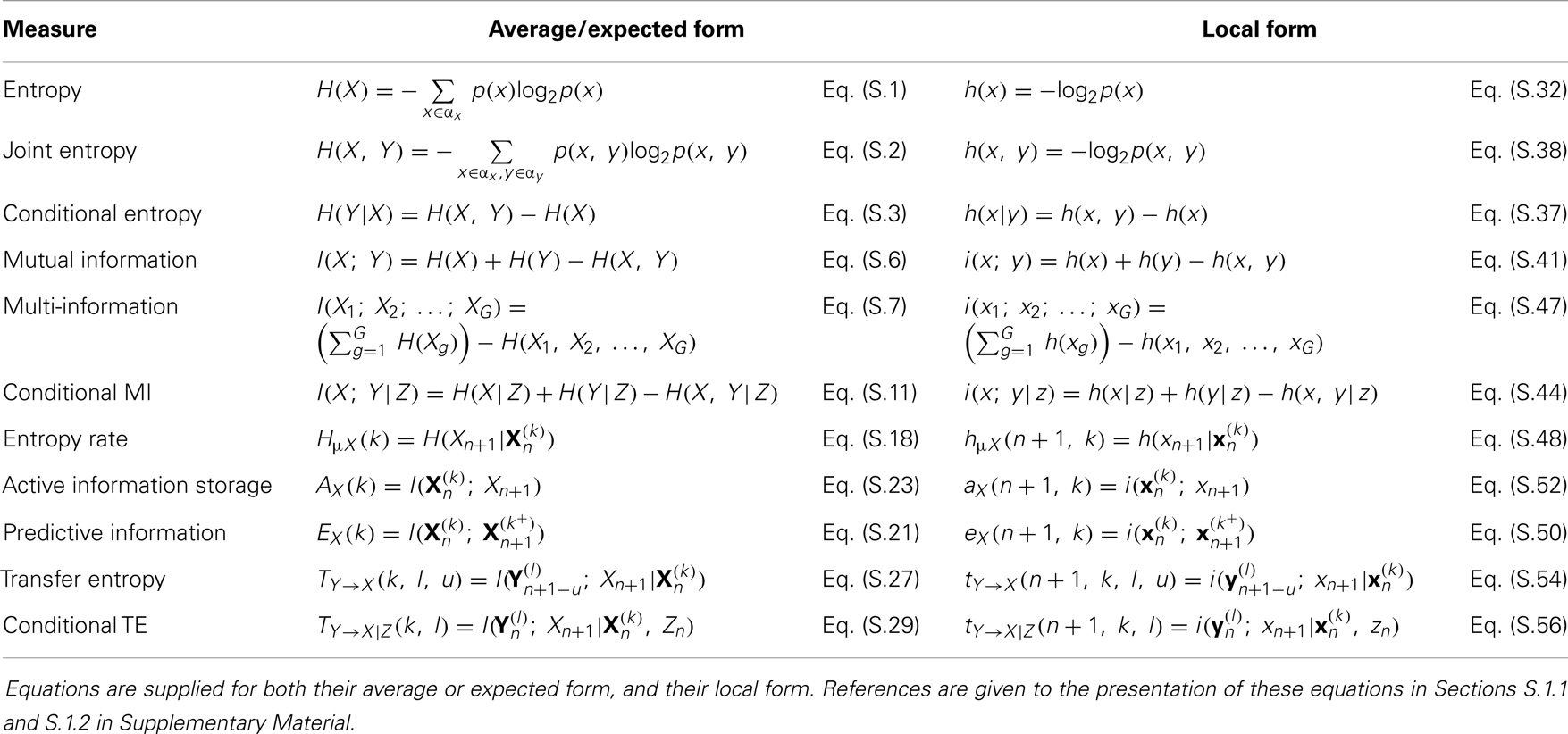
Table 1. Basic information-theoretic quantities (first six measures) and measures of information dynamics (last five measures) implemented in JIDT.

All of the subsequent Shannon information-theoretic quantities we consider may be written as sums and differences of the aforementioned marginal and joint entropies, and all may be extended to multivariate (X, Y, etc.) and/or continuous variables. The basic information-theoretic quantities: entropy, joint entropy, conditional entropy, mutual information (MI), conditional mutual information (Cover and Thomas, 1991; MacKay, 2003), and multi-information (Tononi et al., 1994); are discussed in detail in Section S.1.1 in Supplementary Material, and summarized here in Table 1. All of these measures are non-negative.

Also, we may write down pointwise or local information-theoretic measures, which characterize the information attributed with specific measurements x, y, and z of variables X, Y, and Z (Lizier, 2014), rather than the traditional expected or average information measures associated with these variables introduced above. Full details are provided in Section S.1.3 in Supplementary Material, and the local form for all of our basic measures is shown here in Table 1. For example, the Shannon information content or local entropy of an outcome x of measurement of the variable X is (Ash, 1965; MacKay, 2003):

$h\left(x\right)=-{\text{log}}_{2}p\left(x\right).$ (2)

By convention, we use lower-case symbols to denote local information-theoretic measures. The Shannon information content of a given symbol x is the code-length for that symbol in an optimal encoding scheme for the measurements X, i.e., one that produces the minimal expected code length. We can form all local information-theoretic measures as sums and differences of local entropies (see Table 1; Section S.1.3 in Supplementary Material), and each ordinary measure is the average or expectation value of their corresponding local measure, e.g., H(X) = ⟨h(x)⟩. Crucially, the local MI and local conditional MI (Fano, 1961) may be negative, unlike their averaged forms. This occurs for MI where the measurement of one variable is misinformative about the other variable (see further discussion in Section S.1.3 in Supplementary Material).

Applied to time-series data, these local variants return a time-series for the given information-theoretic measure, which with mutual information, for example, characterizes how the shared information between the variables fluctuates as a function of time. As such, they directly reveal the dynamics of information, and are gaining popularity in complex systems analysis (Shalizi, 2001; Helvik et al., 2004; Shalizi et al., 2006; Lizier et al., 2007, 2008c, 2010, 2012b; Lizier, 2014; Wibral et al., 2014a).

Continuing with time-series, we then turn our attention to measures specifically used to quantify the dynamics of information processing in multivariate time-series, under a framework for information dynamics, which was recently introduced by Lizier et al. (2007, 2008c, 2010, 2012b, 2014) and Lizier (2013, 2014). The measures of information dynamics implemented in JIDT – which are the real focus of the toolkit – are discussed in detail in Section S.1.2 in Supplementary Material, and summarized here in Table 1.

These measures consider time-series processes X of the random variables {… X_n−1, X_n, X_n+1…} with process realizations {… x_n−1, x_n, x_n+1 …} for countable time indices n. We use $X_n^{\left(k\right)}=\left\{X_{n-k+1},\dots ,X_{n-1},X_n\right\}$ to denote the k consecutive variables of X up to and including time step n, which has realizations $x_n^{\left(k\right)}=\left\{x_{n-k+1},\dots ,x_{n-1},x_n\right\}$². The $x_n^{\left(k\right)}$ are Takens’ embedding vectors (Takens, 1981) with embedding dimension k, which capture the underlying state of the process X for Markov processes of order k³.

Specifically, our framework examines how the information in variable X_n+1 is related to previous variables or states (e.g., X_n or $X_n^{\left(k\right)}$) of the process or other related processes, addressing the fundamental question: “where does the information in a random variable X_n+1 in a time series come from?” As indicated in Figure 1 and shown for the respective measures in Table 1, this question is addressed in terms of

1. information from the past of process X – i.e., the information storage, measured by the active information storage (Lizier et al., 2012b), and predictive information or excess entropy (Grassberger, 1986; Bialek et al., 2001; Crutchfield and Feldman, 2003);

2. information contributed from other source processes Y – i.e., the information transfer, measured by the transfer entropy (TE) (Schreiber, 2000), and conditional transfer entropy (Lizier et al., 2008c, 2010);

3. and how these sources combine – i.e., information modification (see separable information (Lizier et al., 2010) in Section S.1.2 in Supplementary Material).

FIGURE 1

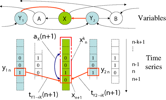
Figure 1. Measures of information dynamics with respect to a destination variable X. We address the information content in a measurement x_n+1 of X at time n + 1 with respect to the active information storage a_X(n + 1, k), and local transfer entropies $t_{Y_1\to X}\left(n+1,k\right)$ and $t_{Y_2\to X}\left(n+1,k\right)$ from variables Y₁ and Y₂.

The goal of the framework is to decompose the information in the next observation X_n+1 of process X in terms of these information sources.

The transfer entropy, arguably the most important measure in the toolkit, has become a very popular tool in complex systems in general, e.g., (Lungarella and Sporns, 2006; Lizier et al., 2008c, 2011c; Obst et al., 2010; Williams and Beer, 2011; Barnett and Bossomaier, 2012; Boedecker et al., 2012), and in computational neuroscience, in particular, e.g., (Ito et al., 2011; Lindner et al., 2011; Lizier et al., 2011a; Vicente et al., 2011; Stramaglia et al., 2012). For multivariate Gaussians, the TE is equivalent (up to a factor of 2) to the Granger causality (Barnett et al., 2009). Extension of the TE to arbitrary source-destination lags is described by Wibral et al. (2013) and incorporated in Table 1 (this is not shown for conditional TE here for simplicity, but is handled in JIDT). Further, one can consider multivariate sources Y, in which case we refer to the measure T_Y→X(k, l) as a collective transfer entropy (Lizier et al., 2010). See further description of this measure at Section S.1.2 in Supplementary Material, including regarding how to set the history length k.

Table 1 also shows the local variants of each of the above measures of information dynamics (presented in full in Section S.1.3 in Supplementary Material). The use of these local variants is particularly important here because they provide a direct, model-free mechanism to analyze the dynamics of how information processing unfolds in time in complex systems. Figure 1 indicates, for example, a local active information storage measurement for time-series process X, and a local transfer entropy measurement from process Y to X.

Finally, in Section S.1.5 in Supplementary Material, we describe how one can evaluate whether an MI, conditional MI, or TE is statistically different from 0, and therefore, represents sufficient evidence for a (directed) relationship between the variables. This is done (following (Chávez et al., 2003; Verdes, 2005; Lindner et al., 2011; Lizier et al., 2011a; Vicente et al., 2011; Barnett and Bossomaier, 2012; Wibral et al., 2014b)) via permutation testing to construct appropriate surrogate populations of time-series and measurements under the null hypothesis of no directed relationship between the given variables.

2.2. Estimation Techniques

While the mathematical formulation of the quantities in Section 2.1 are relatively straightforward, empirically estimating them in practice from a finite number N of samples of time-series data can be a complex process, and is dependent on the type of data you have and its properties. Estimators are typically subject to bias and variance due to finite sample size. Here, we briefly introduce the various types of estimators that are included in JIDT, referring the reader to Section S.2 in Supplementary Material (and also (Vicente and Wibral, 2014) for the transfer entropy, in particular) for more detailed discussion.

For discrete variables X, Y, Z, etc., the definitions in Section 2.1 may be used directly by counting the matching configurations in the available data to obtain the relevant plug-in probability estimates (e.g., $\widehat{p}\left(x|y\right)$ and $\widehat{p}\left(x\right)$ for MI). These estimators are simple and fast, being implemented in O (N) time. Several bias correction techniques are available, e.g., Paninski (2003), Bonachela et al. (2008), though not yet implemented in JIDT.

For continuous variables X, Y, Z, one could simply discretize or bin the data and apply the discrete estimators above. While this is simple and fast (O (N) as above), it is likely to sacrifice accuracy. Alternatively, we can use an estimator that harnesses the continuous nature of the variables, dealing with the differential entropy and probability density functions. The latter is more complicated but yields a more accurate result. We discuss several such estimators in Section S.2.2 in Supplementary Material, and summarize them in the following⁴:

• A multivariate Gaussian model may be used (Section S.2.2.1 in Supplementary Material) for the relevant variables, assuming linear interactions between them. This approach uses the known form of entropy for Gaussian multivariates (equation (S.61) in Supplementary Material, in nats) (Cover and Thomas, 1991) and sums and differences of these entropies to compute other measures (e.g., transfer entropy as per (Kaiser and Schreiber, 2002)). These estimators are fast (O (Nd²), for dimensionality d of the given joint variable) and parameter-free, but subject to the linear-model assumption.

• Kernel estimation of the relevant PDFs via a kernel function are discussed in Section S.2.2.2 in Supplementary Material (and see, e.g., Schreiber (2000), Kaiser and Schreiber (2002), and Kantz and Schreiber (1997)). Such kernel functions measure similarity between pairs of samples using a specific resolution or kernel width r; e.g., the box-kernel (implemented in JIDT) results in counting the proportion of the N sample values, which fall within r of the given sample. They are then used as plug-in estimates for the entropy, and again sums and differences of these for the other measures. Kernel estimation can measure non-linear relationships and is model-free (unlike Gaussian estimators), though is sensitive to the parameter choice for r (Schreiber, 2000; Kaiser and Schreiber, 2002) and is biased. It is less time-efficient than the simple methods, although box-assisted methods can achieve O (N) time-complexity (Kantz and Schreiber, 1997). See Section S.2.2.2 in Supplementary Material for further comments, e.g., regarding selection of r.

• The Kraskov et al. (2004) (KSG) technique (see details in Section S.2.2.3 in Supplementary Material) improved on (box-) kernel estimation for MI (and multi-information) via the use of Kozachenko–Leonenko estimators (Kozachenko and Leonenko, 1987) of log-probabilities via nearest-neighbor counting; bias correction; and a fixed number K of nearest neighbors in the full X-Y joint space. The latter effectively means using a dynamically altered (box-) kernel width r to adjust to the density of samples in the vicinity of any given observation; this smooths out errors in the PDF estimation, especially when handling a small number of observations. These authors proposed two slightly different algorithms for their estimator – both are implemented in JIDT. The KSG technique has been directly extended to conditional MI by Frenzel and Pompe (2007) and transfer entropy (originally by Gomez-Herrero et al. (2010)) and later for algorithm 2 by Wibral et al. (2014b)). KSG estimation builds on the non-linear and model-free capabilities of kernel estimation with bias correction, better data efficiency and accuracy, and being effectively parameter-free (being relatively stable to choice of K). As such, it is widely used as best of breed solution for MI, conditional MI and TE for continuous data; see, e.g., Wibral et al. (2014b) and Vicente and Wibral (2014). It can be computationally expensive with naive algorithms requiring O (KN²) time though fast nearest neighbor search techniques can reduce this to O (KNlogN). For release v1.0 JIDT only implements a naive algorithm, though fast nearest neighbor search is implemented and available via the project SVN repository (see Section 3.1) and as such will be included in future releases.

• Permutation entropy approaches (Bandt and Pompe, 2002) estimate the relevant PDFs based on the relative ordinal structure of the joint vectors (see Section S.2.2.4 in Supplementary Material). Permutation entropy has, for example, been adapted to estimate TE as the symbolic transfer entropy (Staniek and Lehnertz, 2008). Permutation approaches are computationally fast, but are model-based, however, (assuming all relevant information is in the ordinal relationships). This is not necessarily the case, and can lead to misleading results, as demonstrated by Wibral et al. (2013).

2.3. Related Open-Source Information-Theoretic Toolkits

We next consider other existing open-source information-theoretic toolkits for computing the aforementioned measures empirically from time-series data. In particular, we consider those that provide implementations of the transfer entropy. For each toolkit, we describe its purpose, the type of data it handles, and which measures and estimators are implemented.

TRENTOOL⁵ (GPL v3 license) by Lindner et al. (2011) is a MATLAB toolbox, which is arguably the most mature open-source toolkit for computing TE. It is not intended for general-purpose use, but designed from the ground up for transfer entropy analysis of (continuous) neural data, using the data format of the FieldTrip toolbox (Oostenveld et al., 2011) for EEG, MEG, and LFP recordings. In particular, it is designed for performing effective connectivity analysis between the input variables (see Vicente et al. (2011) and Wibral et al. (2011)), including statistical significance testing of TE results (as outlined in Section S.1.5 in Supplementary Material) and processing steps to deal with volume conduction and identify cascade or common-driver effects in the inferred network. Conditional/multivariate TE is not yet available, but planned. TRENTOOL automates selection of parameters for embedding input time-series data and for source-target delays, and implements KSG estimation (see Section S.2.2.3 in Supplementary Material), harnessing fast nearest neighbor search, parallel computation, and GPU-based algorithms (Wollstadt et al., 2014).

The MuTE toolbox by Montalto et al. (2014a,b) (CC-BY license)⁶ provides MATLAB code for TE estimation. In particular, MuTE is capable of computing conditional TE, includes a number of estimator types (discrete or binned, Gaussian, and KSG including fast nearest neighbor search), and adds non-uniform embedding (see Faes et al. (2011)). It also adds code to assist with embedding parameter selection, and incorporates statistical significance testing.

The Transfer entropy toolbox (TET, BSD license)⁷ by Ito et al. (2011) provides C-code callable from MATLAB for TE analysis of spiking data. TET is limited to binary (discrete) data only. Users can specify embedding dimension and source-target delay parameters.

MILCA (Mutual Information Least-dependent Component Analysis, GPL v3 license)⁸ provides C-code (callable from MATLAB) for mutual information calculations on continuous data (Kraskov et al., 2004; Stögbauer et al., 2004; Astakhov et al., 2013). MILCA’s purpose is to use the MI calculations as part of Independent Component Analysis (ICA), but they can be accessed in a general-purpose fashion. MILCA implements KSG estimators with fast nearest neighbor search; indeed, MILCA was co-written by the authors of this technique. It also handles multidimensional variables.

TIM (GNU Lesser GPL license)⁹ by Rutanen (2011) provides C++ code (callable from MATLAB) for general-purpose calculation of a wide range of information-theoretic measures on continuous-valued time-series, including for multidimensional variables. The measures implemented include entropy (Shannon, Renyi, and Tsallis variants), Kullback–Leibler divergence, MI, conditional MI, TE, and conditional TE. TIM includes various estimators for these, including Kozachenko–Leonenko (see Section S.2.2.3 in Supplementary Material), Nilsson and Kleijn (2007), and Stowell and Plumbley (2009) estimators for (differential) entropy, and KSG estimation for MI and conditional MI (using fast nearest neighbor search).

The MVGC (multivariate Granger causality toolbox, GPL v3 license)¹⁰ by Barnett and Seth (2014) provides a MATLAB implementation for general-purpose calculation of the Granger causality (i.e., TE with a linear-Gaussian model, see Section S.1.2 in Supplementary Material) on continuous data. MVGC also requires the MATLAB Statistics, Signal Processing, and Control System Toolboxes.

There is a clear gap for a general-purpose information-theoretic toolkit, which can run in multiple code environments, implementing all of the measures in Sections S.1.1 and S.1.2 in Supplementary Material, with various types of estimators, and with implementation of local values, measures of statistical significance, etc. In the next section, we introduce JIDT, and outline how it addresses this gap. Users should make a judicious choice of which toolkit suits their requirements, taking into account data types, estimators and application domain. For example, TRENTOOL is built from the ground up for effective network inference in neural imaging data, and is certainly the best tool for that application in comparison to a general-purpose toolkit.

3. JIDT Installation, Contents, and Design

JIDT (Java Information Dynamics Toolkit, GPL v3 license)¹¹ is unique as a general-purpose information-theoretic toolkit, which provides all of the following features in one package:

• Implementation of a large array of measures, including all conditional/multivariate forms of the transfer entropy, complementary measures such as active information storage, and allows full specification of relevant embedding parameters;

• Implementation a wide variety of estimator types and applicability to both discrete and continuous data;

• Implementation of local measurement for all estimators;

• Inclusion of statistical significance calculations for MI, TE, etc., and their conditional variants;

• No dependencies on other installations (except Java).

Furthermore, JIDT is written in Java¹², taking advantage of the following features:

• The code becomes platform agnostic, requiring only an installation of the Java Virtual Machine (JVM) to run;

• The code is object-oriented, with common code shared and an intuitive hierarchical design using interfaces; this provides flexibility and allows different estimators of same measure can be swapped dynamically using polymorphism;

• The code can be called directly from MATLAB, GNU Octave, Python, etc., but runs faster than native code in those languages (still slower but comparable to C/C++, see Computer Language Benchmarks Game, 2014); and

• Automatic generation of Javadoc documents for each class.

In the following, we describe the (minimal) installation process in Section 3.1, and contents of the version 1.0 JIDT distribution in Section 3.2. We then describe which estimators are implemented for each measure in Section 3.3, and architecture of the source code in Section 3.4. We also outline how the code has been tested in Section 3.5, how to build it (if required) in Section 3.6 and point to other sources of documentation in Section 3.7.

3.1. Installation and Dependencies

There is little to no installation of JIDT required beyond downloading the software. The software can be run on any platform, which supports a standard edition Java Runtime Environment (i.e., Windows, Mac, Linux, and Solaris).

Material pertaining to installation is described in full at the “Installation” wiki page for the project (see Table 2 for all relevant project URLs); summarized as follows:

1. Download a code release package from the “Downloads” wiki page. Full distribution is recommended (described in Section 3.2) so as to obtain, e.g., access to the examples described in Section 4, though a “Jar only” distribution provides just the JIDT library infodynamics.jar in Java archive file format.

2. Unzip the full .zip distribution to the location of your choice, and/or move the infodynamics.jar file to a relevant location. Ensure that infodynamics.jar is on the Java classpath when your code attempts to access it (see Section 4).

3. To update to a new version, simply copy the new distribution over the top of the previous one.

TABLE 2

Table 2. Relevant web/wiki pages on JIDT website.

As an alternative, advanced users can take an SVN checkout of the source tree from the SVN URL (see Table 2) and build the infodynamics.jar file using ant scripts (see Section 3.6).

In general, there are no dependencies that a user would need to download in order to run the code. Some exceptions are as follows:

1. Java must be installed on your system in order to run JIDT; most systems will have Java already installed. To simply run JIDT, you will only need a Java Runtime Environment (JRE, also known as Java Virtual Machine or JVM), whereas to modify and/or build to software, or write your own Java code to access it, you will need the full Java Development Kit (JDK), standard edition (SE). Download it from http://java.com/. For using JIDT via MATLAB, a JVM is included in MATLAB already.

2. If you wish to build the project using the build.xml script – this requires ant (see Section 3.6).

3. If you wish to run the unit test cases (see Section 3.5) – this requires the JUnit framework: http://www.junit.org/ – for how to run JUnit with our ant script see “JUnit test cases” wiki page.

4. Additional preparation may be required to use JIDT in GNU Octave or Python. Octave users must install the octave-java package from the Octave-forge project – see description of these steps at “MATLAB/Octave use” wiki page. Python users must install a relevant Python-Java extension – see description at “Python use” wiki page. Both cases will depend on a JVM on the system (as per point 1 above), though the aforementioned extensions may install this for you.

Note that JIDT does adapt code from a number of sources in accordance with their open-source license terms, including Apache Commons Math v3.3¹³, the JAMA project¹⁴, and the octave-java package from the Octave-Forge project¹⁵. Relevant notices are supplied in the notices folder of the distribution. Such code is included in JIDT, however, and does not need to be installed separately.

3.2. Contents of Distribution

The contents of the current (version 1.0) JIDT (full) distribution are as follows:

• The top-level folder contains the infodynamics.jar library file, a GNU GPL v3 license, a readme.txt file and an ant build.xml script for (re-)building the code (see Section 3.6);

• The java folder contains source code for the library in the source subfolder (described in Section 3.3), and unit tests in the unittests subfolder (see Section 3.5).

• The javadocs folder contains automatically generated Javadocs from the source code, as discussed in Section 3.7.

• The demos folder contains several example applications of the software, described in Section 4, sorted into folders to indicate that environment they are intended to run in, i.e., java, octave (which is compatible with MATLAB), and python. There is also a data folder here containing sample data sets for these demos and unit tests.

• The notices folder contains notices and licenses pertaining to derivations of other open-source code used in this project.

3.3. Source Code and Estimators Implemented

The Java source code for the JIDT library contained in the java/source folder is organized into the following Java packages (which map directly to subdirectories):

• infodynamics.measures contains all of the classes implementing the information-theoretic measures, split into:

• infodynamics.measures.discrete containing all of the measures for discrete data;

• infodynamics.measures.continuous which at the top-level contains Java interfaces for each of the measures as applied to continuous data, then a set of sub-packages (gaussian, kernel, kozachenko, kraskov, and symbolic), which map to each estimator type in Section 2.2 and contain implementations of such estimators for the interfaces defined for each measure (Section 3.4 describes the object-oriented design used here). Table 3 identifies which estimators are measured for each estimator type;

• infodynamics.measures.mixed includes experimental discrete-to-continuous MI calculators, though these are not discussed in detail here.

• infodynamics.utils contains classes providing a large number of utility functions for the measures (e.g., matrix manipulation, file reading/writing including in Octave text format);

• infodynamics.networkinference contains implementations of higher-level algorithms, which use the information-theoretic calculators to infer an effective network structure from time-series data (see Section 4.6).

TABLE 3

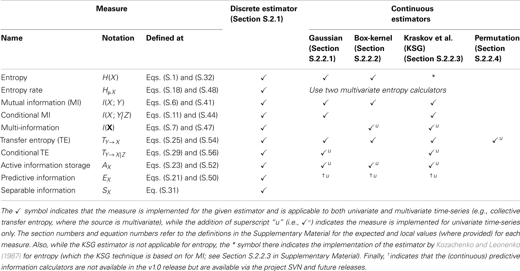
Table 3. An outline of which estimation techniques are implemented for each relevant information-theoretic measure.

As outlined above, Table 3 describes which estimators are implemented for each measure. This effectively maps the definitions of the measures in Section 2.1 to the estimators in Section 2.2 (note that the efficiency of these estimators is also discussed in Section 2.1). All estimators provide the corresponding local information-theoretic measures (as introduced in Section S.1.3 in Supplementary Material). Also, for the most part, the estimators include a generalization to multivariate X, Y, etc., as identified in the table.

3.4. JIDT Architecture

The measures for continuous data have been organized in a strongly object-oriented fashion¹⁶. Figure 2 provides a sample (partial) Unified Modeling Language (UML) class diagram of the implementations of the conditional mutual information (equation (S.11) in Supplementary Material) and transfer entropy (equation (S.25) in Supplementary Material) measures using KSG estimators (Section S.2.2.3 in Supplementary Material). This diagram shows the typical object-oriented hierarchical structure of the implementations of various estimators for each measure. The class hierarchy is organized as follows.

FIGURE 2

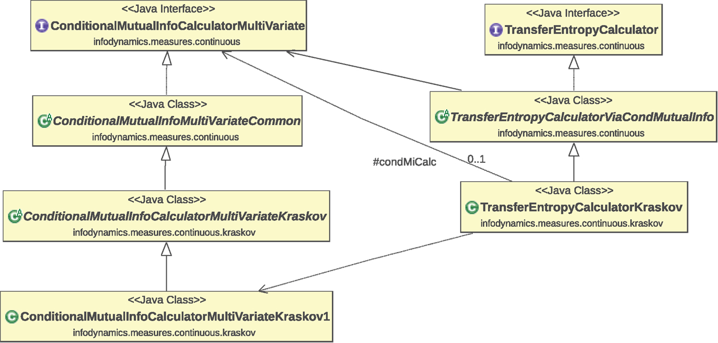
Figure 2. Partial UML class diagram of the implementations of the conditional mutual information (equation (S.11) in Supplementary Material) and transfer entropy (equation (S.25) in Supplementary Material) measures using KSG estimators. As explained in the main text, this diagram shows the typical object-oriented structure of the implementations of various estimators for each measure. The relationships indicated on the class diagram are as follows: dotted lines with hollow triangular arrow heads indicate the realization or implementation of an interface by a class; solid lines with hollow triangular arrow heads indicate the generalization or inheritance of a child or subtype from a parent or superclass; lines with plain arrow heads indicate that one class uses another (with the solid line indicating direct usage and dotted line indicating indirect usage via the superclass).

3.4.1. Interfaces

Interfaces at the top layer define the available methods for each measure. At the top of this figure we see the ConditionalMutualInfoCalculatorMultiVariate and TransferEntropyCalculator interfaces, which define the methods each estimator class for a given measure must implement. Such interfaces are defined for each information-theoretic measure in the infodynamics.measures.continuous package.

3.4.2. Abstract classes

Abstract classes¹⁷ at the intermediate layer provide basic functionality for each measure. Here, we have abstract classes ConditionalMutualInfoMultiVariateCommon and TransferEntropyCalculatorViaCondMutualInfo which implement the above interfaces, providing common code bases for the given measures that various child classes can build on to specialize themselves to a particular estimator type. For instance, the TransferEntropyCalculatorViaCondMutualInfo class provides code which abstractly uses a ConditionalMutualInfoCalculatorMultiVariate interface in order to make transfer entropy calculations, but neither concretely specify which type of conditional MI estimator to use nor fully set its parameters.

3.4.3. Child classes

Child classes at the lower layers add specialized functionality for each estimator type for each measure. These child classes inherit from the above parent classes, building on the common code base to add specialization code for the given estimator type. Here, that is the KSG estimator type. The child classes at the bottom of the hierarchy have no remaining abstract functionality, and can thus be used to make the appropriate information-theoretic calculation. We see that ConditionalMutualInfoCalculatorMultiVariateKraskov begins to specialize ConditionalMutualInfoMultiVariateCommon for KSG estimation, with further specialization by its child class ConditionalMutualInfoCalculatorMultiVariateKraskov1 which implements the KSG algorithm 1 (equation (S.64) in Supplementary Material). Not shown here is ConditionalMutualInfoCalculatorMultiVariateKraskov2 which implements the KSG algorithm 2 (equation (S.65) in Supplementary Material) and has similar class relationships. We also see that TransferEntropyCalculatorKraskov specializes TransferEntropyCalculatorViaCondMutualInfo for KSG estimation, by using ConditionalMutualInfoCalculatorMultiVariateKraskov1 (or ConditionalMutuaInfoCalculatorMultiVariateKraskov2, not shown) as the specific implementation of ConditionalMutualInfoCalculatorMultiVariate. The implementations of these interfaces for other estimator types (e.g., TransferEntropyCalculatorGaussian) sit at the same level here inheriting from the common abstract classes above.

This type of object-oriented hierarchical structure delivers two important benefits: (i) the decoupling of common code away from specific estimator types and into common parent classes allows code re-use and simpler maintenance, and (ii) the use of interfaces delivers subtype polymorphism allowing dynamic dispatch, meaning that one can write code to compute a given measure using the methods on its interface and only specify the estimator type at runtime (see a demonstration in Section 4.1.8).

3.5. Validation

The calculators in JIDT are validated using a set of unit tests (distributed in the java/unittests folder). Unit testing is a method of testing software by the use of a set of small test cases which call parts of the code and check the output against expected values, flagging errors if they arise. The unit tests in JIDT are implemented via the JUnit framework version 3¹⁸. They can be run via the ant script (see Section 3.6).

At a high level, the unit tests include validation of the results of information-theoretic calculations applied to the sample data in demos/data against measurements from various other existing toolkits, e.g.,

• The KSG estimator (Section S.2.2.3 in Supplementary Material) for MI is validated against values produced from the MILCA toolkit (Kraskov et al., 2004; Stögbauer et al., 2004; Astakhov et al., 2013);

• The KSG estimator for conditional MI and TE is validated against values produced from scripts within TRENTOOL (Lindner et al., 2011);

• The discrete and box-kernel estimators for TE are validated against the plots in the original paper on TE by Schreiber (2000) (see Section 4.4);

• The Gaussian estimator for TE (Section S.2.2.1 in Supplementary Material) is verified against values produced from (a modified version of) the computeGranger.m script of the ChaLearn Connectomics Challenge Sample Code (Orlandi et al., 2014).

Further code coverage by the unit tests is planned in future work.

3.6. (Re-)Building the Code

Users may wish to build the code, perhaps if they are directly accessing the source files via SVN or modifying the files. The source code may be compiled manually of course, or in your favorite IDE (Integrated Development Environment). JIDT also provides an ant build script, build.xml, to guide and streamline this process. Apache ant – see http://ant.apache.org/ – is a command-line tool to build various interdependent targets in software projects, much like the older style Makefile for C/C++.

To build any of the following targets using build.xml, either integrate build.xml into your IDE and run the selected <targetName >, or run ant <targetName > from the command line in the top-level directory of the distribution, where <targetName > may be any of the following:

• buildor jar(this is the default if no <targetName > is supplied) – creates a jar file for the JIDT library;

• compile – compiles the JIDT library and unit tests;

• junit – runs the unit tests;

• javadocs – generates automated Javadocs from the formatted comments in the source code;

• jardist – packages the JIDT jar file in a distributable form, as per the jar-only distributions of the project;

• dist – runs unit tests, and packages the JIDT jar file, Javadocs, demos, etc., in a distributable form, as per the full distributions of the project;

• clean – delete all compiled code, etc., built by the above commands.

3.7. Documentation and Support

Documentation to guide users of JIDT is composed of

1. This manuscript!

2. The Javadocs contained in the javadocs folder of the distribution (main page is index.html), and available online via the Documentation page of the project wiki (see Table 2). Javadocs are html formatted documentation for each package, class, and interface in the library, which are automatically created from formatted comments in the source code. The Javadocs are very useful tools for users, since they provide specific details about each class and their methods, in more depth than we are able to do here; for example, which properties may be set for each class. The Javadocs can be (re-)generated using ant as described in Section 3.6.

3. The demos; as described further in Section 4, on the Demos wiki page (see Table 2), and the individual wiki page for each demo;

4. The project wiki pages (accessed from the project home page, see Table 2) provide additional information on various features, e.g., how to use JIDT in MATLAB or Octave and Python;

5. The unit tests (as described in Section 3.5) provide additional examples on how to run the code.

You can also join our email discussion group jidt-discuss on Google Groups (see URL in Table 2) or browse past messages, for announcements, asking questions, etc.

4. JIDT Code Demonstrations

In this section, we describe some simple demonstrations on how to use the JIDT library. Several sets of demonstrations are included in the JIDT distribution, some of which are described here. More detail is provided for each demo on its wiki page, accessible from the main Demos wiki page (see Table 2). We begin with the main set of Simple Java Demos, focusing, in particular, on a detailed walk-through of using a KSG estimator to compute transfer entropy since the calling pattern here is typical of all estimators for continuous data. Subsequently, we provide more brief overviews of other examples available in the distribution, including how to run the code in MATLAB, GNU Octave, and Python, implementing the transfer entropy examples from Schreiber (2000), and computing spatiotemporal profiles of information dynamics in Cellular Automata.

4.1. Simple Java Demos

The primary set of demos is the “Simple Java Demos” set at demos/java in the distribution. This set contains eight standalone Java programs to demonstrate simple use of various aspects of the toolkit. This set is described further at the SimpleJavaExamples wiki page (see Table 2).

The Java source code for each program is located at demos/java/infodynamics/demos in the JIDT distribution, and shell scripts (with mirroring batch files for Windows)¹⁹ to run each program are found at demos/java/. The shell scripts demonstrate how to compile and run the programs from command line, e.g., example1TeBinaryData.sh contains the following commands in Listing 1:

Listing 1. Shell script example1TeBinaryData.sh.

# Make sure the latest source file is compiled.
javac -classpath "../../infodynamics.jar" "infodynamics/demos/Example1TeBinaryData.java"
# Run the example:
java -classpath ".:../../infodynamics.jar" infodynamics.demos.Example1TeBinaryData

The examples focus on various transfer entropy estimators (though similar calling paradigms can be applied to all estimators), including

1. computing transfer entropy on binary (discrete) data;

2. computing transfer entropy for specific channels within multidimensional binary data;

3. computing transfer entropy on continuous data using kernel estimation;

4. computing transfer entropy on continuous data using KSG estimation;

5. computing multivariate transfer entropy on multidimensional binary data;

6. computing mutual information on continuous data, using dynamic dispatch or late-binding to a particular estimator;

7. computing transfer entropy from an ensemble of time-series samples;

8. computing transfer entropy on continuous data using binning then discrete calculation.

In the following, we explore selected salient examples in this set. We begin with Example1TeBinaryData.java and Example4TeContinuousDataKraskov.java as typical calling patterns to use estimators for discrete and continuous data, respectively, then add extensions for how to compute local measures and statistical significance, use ensembles of samples, handle multivariate data and measures, and dynamic dispatch.

4.1.1. Typical calling pattern for an information-theoretic measure on discrete data

Example1TeBinaryData.java (see Listing 2) provides a typical calling pattern for calculators for discrete data, using the infodynamics.measures.discrete.TransferEntropyCalculatorDiscrete class. While the specifics of some methods may be slightly different, the general calling paradigm is the same for all discrete calculators.

Listing 2. Estimation of TE from discrete data; source code adapted from Example1TeBinaryData.java.

int arrayLengths = 100;
RandomGenerator rg = new RandomGenerator();
// Generate some random binary data:
int[] sourceArray = rg.generateRandomInts(arrayLengths, 2);
int[] destArray = new int[arrayLengths];
destArray[0] = 0;
System.arraycopy(sourceArray, 0, destArray, 1, arrayLengths - 1);
// Create a TE calculator and run it:
TransferEntropyCalculatorDiscrete teCalc = new TransferEntropyCalculatorDiscrete(2, 1);
teCalc.initialise();
teCalc.addObservations(sourceArray, destArray);
double result = teCalc.computeAverageLocalOfObservations();

The data type used for all discrete data are int[] time-series arrays (indexed by time). Here, we are computing TE for univariate time series data, so sourceArray and destArray at line 4 and line 5 are single dimensional int[] arrays. Multidimensional time series are discussed in Section 4.1.6.

The first step in using any of the estimators is to construct an instance of them, as per line 9 above. Parameters/properties for calculators for discrete data are only supplied in the constructor at line 9 (this is not the case for continuous estimators, see Section 4.1.2). See the Javadocs for each calculator for descriptions of which parameters can be supplied in their constructor. The arguments for the TE constructor here include the number of discrete values (M = 2), which means the data can take values {0, 1} (the allowable values are always enumerated 0, … , M − 1); and the embedded history length k = 1. Note that for measures such as TE and AIS, which require embeddings of time-series variables, the user must provide the embedding parameters here.

All calculators must be initialized before use or re-use on new data, as per the call to initialise() at line 10. This call clears any PDFs held inside the class, The initialise() method provides a mechanism by which the same object instance may be used to make separate calculations on multiple data sets, by calling it in between each application (i.e., looping from line 12 back to line 10 for a different data set – see the full code for Example1TeBinaryData.java for an example).

The user then supplies the data to construct the PDFs with which the information-theoretic calculation is to be made. Here, this occurs at line 11 by calling the addObservations() method to supply the source and destination time series values. This method can be called multiple times to add multiple sample time-series before the calculation is made (see further commentary for handling ensembles of samples in Section 4.1.5).

Finally, with all observations supplied to the estimator, the resulting transfer entropy may be computed via computeAverageLocalOfObservations() at line 12. The information-theoretic measurement is returned in bits for all discrete calculators. In this example, since the destination copies the previous value of the (randomized) source, then result should approach 1 bit.

4.1.2. Typical calling pattern for an information-theoretic measure on continuous data

Before outlining how to use the continuous estimators, we note that the discrete estimators above may be applied to continuous double[] data sets by first binning them to convert them to int[] arrays, using either MatrixUtils.discretise(double data[], int numBins) for even bin sizes or MatrixUtils.discretiseMaxEntropy(double data[], int numBins) for maximum entropy binning (see Example8TeContinuousDataByBinning). This is very efficient, however, as per section 2.2 it is more accurate to use an estimator, which utilizes the continuous nature of the data.

As such, we now review the use of a KSG estimator (Section S.2.2.3 in Supplementary Material) to compute transfer entropy (equation (S.25) in Supplementary Material), as a standard calling pattern for all estimators applied to continuous data. The sample code in Listing 3 is adapted from Example4TeContinuousDataKraskov.java. (That this is a standard calling pattern can easily be seen by comparing to Example3TeContinuousDataKernel.java, which uses a box-kernel estimator but has very similar method calls, except for which parameters are passed in).

Listing 3. Use of KSG estimator to compute transfer entropy; adapted from Example4TeContinuousDataKraskov.java.

double[] sourceArray, destArray;
// ...
// Import values into sourceArray and destArray
// ...
TransferEntropyCalculatorKraskov teCalc = new TransferEntropyCalculatorKraskov();
teCalc.setProperty("k", "4");
teCalc.initialise(1);
teCalc.setObservations(sourceArray, destArray);
double result = teCalc. computeAverageLocalOfObservations();

Notice that the calling pattern here is almost the same as that for discrete calculators, as seen in Listing 2, with some minor differences outlined below.

Of course, for continuous data we now use double[] arrays (indexed by time) for the univariate time-series data here at line 1. Multidimensional time series are discussed in Section 4.1.7.

As per discrete calculators, we begin by constructing an instance of the calculator, as per line 5 above. Here, however, parameters for the operation of the estimator are not only supplied via the constructor (see below). As such, all classes offer a constructor with no arguments, while only some implement constructors which accept certain parameters for the operation of the estimator.

Next, almost all relevant properties or parameters of the estimators can be supplied by passing key-value pairs of String objects to the setProperty(String, String) method at line 6. The key values for properties, which may be set for any given calculator are described in the Javadocs for the setProperty method for each calculator. Properties for the estimator may be set by calling setProperty at any time; in most cases, the new property value will take effect immediately, though it is only guaranteed to hold after the next initialization (see below). At line 6, we see that property “k” (shorthand for ConditionalMutualInfoCalculatorMultiVariateKraskov.PROP_K) is set to the value “4.” As described in the Javadocs for TransferEntropyCalculatorKraskov.setProperty, this sets the number of nearest neighbors K to use in the KSG estimation in the full joint space. Properties can also easily be extracted and set from a file, see Example6LateBindingMutualInfo.java.

As per the discrete calculators, all continuous calculators must be initialized before use or re-use on new data (see line 7). This clears any PDFs held inside the class, but additionally finalizes any property settings here. Also, the initialise() method for continuous estimators may accept some parameters for the calculator – here, it accepts a setting for the k embedded history length parameter for the transfer entropy (see equation (S.25) in Supplementary Material). Indeed, there may be several overloaded forms of initialise() for a given class, each accepting different sets of parameters. For example, the TransferEntropyCalculatorKraskov used above offers an initialise(k, tau_k, l, tau_l, u) method taking arguments for both source and target embedding lengths k and l, embedding delays τ_k and τ_l (see Section S.1.2 in Supplementary Material), and source-target delay u (see equation (S.27) in Supplementary Material). Note that currently such embedding parameters must be supplied by the user, although we intend to implement automated embedding parameter selection in the future. Where a parameter is not supplied, the value given for it in a previous call to initialise() or setProperty() (or otherwise its default value) is used.

The supply of samples is also subtly different for continuous estimators. Primarily, all estimators offer the setObservations() method (line 8) for supplying a single time-series of samples (which can only be done once). See Section 4.1.5 for how to use multiple time-series realizations to construct the PDFs via an addObservations() method.

Finally, the information-theoretic measurement (line 9) is returned in either bits or nats as per the standard definition for this type of estimator in Section 2.2 (i.e., bits for discrete, kernel, and permutation estimators; nats for Gaussian and KSG estimators).

At this point (before or after line 9) once all observations have been supplied, there are other quantities that the user may compute. These are described in the next two subsections.

4.1.3. Local information-theoretic measures

Listing 4 computes the local transfer entropy (equation (S.54) in Supplementary Material) for the observations supplied earlier in Listing 3:

Listing 4. Computing local measures after Listing 3; adapted from Example4TeContinuousDataKraskov.java.

double[] localTE = teCalc.computeLocalOfPreviousObservations();

Each calculator (discrete or continuous) provides a computeLocalOfPreviousObservations() method to compute the relevant local quantities for the given measure (see Section S.1.3 in Supplementary Material). This method returns a double[] array of the local values (local TE here) at every time step n for the supplied time-series observations. For TE estimators, note that the first k values (history embedding length) will have value 0, since local TE is not defined without the requisite history being available²⁰.

4.1.4. Null distribution and statistical significance

For the observations supplied earlier in Listing 3, Listing 5 computes a distribution of surrogate TE values obtained via resampling under the null hypothesis that sourceArray and destArray have no temporal relationship (as described in Section S.1.5 in Supplementary Material).

Listing 5. Computing null distribution after Listing 3; adapted from Example3TeContinuousDataKernel.java.

EmpiricalMeasurementDistribution dist = teCalc.computeSignificance(1000);

The method computeSignificance() is implemented for all MI and conditional MI based measures (including TE), for both discrete and continuous estimators. It returns an EmpiricalMeasurementDistribution object, which contains a double[] array distribution of an empirical distribution of values obtained under the null hypothesis (the sample size for this distribution is specified by the argument to computeSignificance()). The user can access the mean and standard deviation of the distribution, a p-value of whether these surrogate measurements were greater than the actual TE value for the supplied source, and a corresponding t-score (which assumes a Gaussian distribution of surrogate scores) via method calls on this object (see Javadocs for details).

Some calculators (discrete and Gaussian) overload the method computeSignificance() (without an input argument) to return an object encapsulating an analytically determined p-value of surrogate distribution where this is possible for the given estimation type (see Section S.1.5 in Supplementary Material). The availability of this method is indicated when the calculator implements the AnalyticNullDistributionComputer interface.

4.1.5. Ensemble approach: using multiple trials or realizations to construct PDFs

Now, the use of setObservations() for continuous estimators implies that the PDFs are computed from a single stationary time-series realization. One may supply multiple time-series realizations (e.g., as multiple stationary trials from a brain-imaging experiment) via the following alternative calling pattern to line 8 in Listing 3:

Listing 6. Supply of multiple time-series realizations as observations for the PDFs; an alternative to line 8 in Listing 3. Code is adapted from Example7EnsembleMethodTeContinuousDataKraskov.java.

teCalc.startAddObservations();
teCalc.addObservations(sourceArray1, destArray1);
teCalc.addObservations(sourceArray2, destArray2);
teCalc.addObservations(sourceArray3, destArray3);
// ...
teCalc.finaliseAddObservations();

Computations on the PDFs constructed from this data can then follow as before. Note that other variants of addObservations() exist, e.g., which pull out sub-sequences from the time series arguments; see the Javadocs for each calculator to see the options available. Also, for the discrete estimators, addObservations() may be called multiple times directly without the use of a startAddObservations() or finaliseAddObservations() method. This type of calling pattern may be used to realize an ensemble approach to constructing the PDFs (see Gomez-Herrero et al. (2010), Wibral et al. (2014b), Lindner et al. (2011), and Wollstadt et al. (2014)), in particular, by supplying only short corresponding (stationary) parts of each trial to generate the PDFs for that section of an experiment.

4.1.6. Joint-variable measures on multivariate discrete data

For calculations involving joint variables from multivariate discrete data time-series (e.g., collective transfer entropy, see Section S.1.2 in Supplementary Material), we use the same discrete calculators (unlike the case for continuous-valued data in Section 4.1.7). This is achieved with one simple pre-processing step, as demonstrated by Example5TeBinaryMultivarTransfer.java:

Listing 7. Java source code adapted from Example5TeBinaryMultivarTransfer.java.

int[][] source, dest;
// ...
// Import binary values into the arrays,
// with two columns each.
// ...
TransferEntropyCalculatorDiscrete teCalc = new TransferEntropyCalculatorDiscrete(4, 1);
teCalc.initialise();
teCalc.addObservations(
 MatrixUtils.computeCombinedValues(source, 2),
 MatrixUtils.computeCombinedValues(dest, 2));
double result = teCalc.computeAverageLocalOfObservations();

We see that the multivariate discrete data is represented using two-dimensional int [][] arrays at line 1, where the first array index (row) is time and the second (column) is variable number.

The important pre-processing at line 9 and line 10 involves combining the joint vector of discrete values for each variable at each time step into a single discrete number, i.e., if our joint vector source[t] at time t has v variables, each with M possible discrete values, then we can consider the joint vector as a v-digit base-M number, and directly convert this into its decimal equivalent. The computeCombinedValues() utility in infodynamics.utils.MatrixUtils performs this task for us at each time step, taking the int [][] array and the number of possible discrete values for each variable M = 2 as arguments. Note also that when the calculator was constructed at line 6, we need to account for the total number of possible combined discrete values, being M^v = 4 here.

4.1.7. Joint-variable measures on multivariate continuous data

For calculations involving joint variables from multivariate continuous data time-series, JIDT provides separate calculators to be used. Example6LateBindingMutualInfo.java demonstrates this for calculators implementing the MutualInfoCalculatorMultiVariate interface²¹:

Listing 8. Java source code adapted from Example6LateBindingMutualInfo.java.

double[][] variable1, variable2;
MutualInfoCalculatorMultiVariate miCalc;
// ...
// Import continuous values into the arrays
// and instantiate miCalc
// ...
miCalc.initialise(2, 2);
miCalc.setObservations(variable1, variable2);
double miValue = miCalc.computeAverageLocalOfObservations();

First, we see that the multivariate continuous data is represented using two-dimensional double [][] arrays at line 1, where (as per section 4.1.6) the first array index (row) is time and the second (column) is variable number. The instantiating of a class implementing the MutualInfoCalculatorMultiVariate interface to make the calculations is not shown here (but is discussed separately in Section 4.1.8).

Now, a crucial step in using the multivariate calculators is specifying in the arguments to initialise() the number of dimensions (i.e., the number of variables or columns) for each variable involved in the calculation. At line 7, we see that each variable in the MI calculation has two dimensions (i.e., there will be two columns in each of variable1 and variable2).

Other interactions with these multivariate calculators follow the same form as for the univariate calculators.

4.1.8. Coding to interfaces; or dynamic dispatch

Listing 8 (Example6LateBindingMutualInfo.java) also demonstrates the manner in which a user can write code to use the interfaces defined in infodynamics.measures.continuous – rather than any particular class implementing that measure – and dynamically alter the instantiated class implementing this interface at runtime. This is known as dynamic dispatch, enabled by the polymorphism provided by the interface (described at Section 3.4). This is a useful feature in object-oriented programing where, here, a user wishes to write code which requires a particular measure, and dynamically switch-in different estimators for that measure at runtime. For example, in Listing 8, we may normally use a KSG estimator, but switch-in a linear-Gaussian estimator if we happen to know our data is Gaussian.

To use dynamic dispatch with JIDT:

1. Write code to use an interface for a calculator (e.g., MutualInfoCalculatorMultiVariate in Listing 8), rather than to directly use a particular implementing class (e.g., MutualInfoCalculatorMultiVariateKraskov);

2. Instantiate the calculator object by dynamically specifying the implementing class (compare to the static instantiation at line 5 of Listing 3), e.g., using a variable name for the class as shown in Listing 9:

Listing 9. Dynamic instantiation of a mutual information calculator, belonging at line 5 in Listing 8. Adapted from Example6LateBindingMutualInfo.java.

String implementingClass;
// Load the name of the class to be used into
// the variable implementingClass
miCalc = (MutualInfoCalculatorMultiVariate) Class.forName(implementingClass).newInstance();

Of course, to be truly dynamic, the value of implementingClass should not be hard-coded but must be somehow set by the user. For example, in the full Example6LateBindingMutualInfo.java it is set from a properties file.

4.2. MATLAB/Octave Demos

The “Octave/MATLAB code examples” set at demos/octave in the distribution provide a basic set of demonstration scripts for using the toolkit in GNU Octave or MATLAB. The set is described in some detail at the OctaveMatlabExamples wiki page (Table 2). See Section 3.1 regarding installation requirements for running the toolkit in Octave, with more details at the UseInOctaveMatlab wiki page (see Table 2).

The scripts in this set mirror the Java code in the “Simple Java Demos” set (Section 4.1), to demonstrate that anything which JIDT can do in a Java environment can also be done in MATLAB/Octave. The user is referred to the distribution or the OctaveMatlabExamples wiki page for more details on the examples. An illustrative example is provided in Listing 10, which converts Listing 2 into MATLAB/Octave:

Listing 10. Estimation of TE from discrete data in MATLAB/Octave; adapted from example1TeBinaryData.m.

javaaddpath(’../../infodynamics.jar’);
sourceArray=(rand(100,1)>0.5)*1;
destArray = [0; sourceArray(1:99)];
teCalc=javaObject(’infodynamics.measures.discrete.TransferEntropyCalculatorDiscrete’, 2, 1);
teCalc.initialise();
teCalc.addObservations(
 octaveToJavaIntArray(sourceArray),
 octaveToJavaIntArray(destArray));
result = teCalc.computeAverageLocalOfObservations()

This example illustrates several important steps for using JIDT from a MATLAB/Octave environment:

1. Specify the classpath (i.e., the location of the infodynamics.jar library) before using JIDT with the function javaaddpath(samplePath) (at line 1);

2. Construct classes using the javaObject() function (see line 4);

3. Use of objects is otherwise almost the same as in Java itself, however,

a. In Octave, conversion between native array data types and Java arrays is not straightforward; we recommend using the supplied functions for such conversion in demos/octave, e.g., octaveToJavaIntArray.m. These are described on the OctaveJavaArrayConversion wiki page (Table 2), and see example use in line 7 here, and in example2TeMultidimBinaryData.m and example5TeBinaryMultivarTransfer.m.

b. In Java arrays are indexed from 0, whereas in Octave or MATLAB these are indexed from 1. So when you call a method on a Java object such as MatrixUtils.select(double data, int fromIndex, int length) – even from within MATLAB/Octave – you must be aware that fromIndex will be indexed from 0 inside the toolkit, not 1!

4.3. Python Demos

Similarly, the “Python code examples” set at demos/pythonin the distribution provide a basic set of demonstration scripts for using the toolkit in Python. The set is described in some detail at the PythonExamples wiki page (Table 2). See Section 3.1 regarding installation requirements for running the toolkit in Python, with more details at the UseInPythonwiki page (Table 2).

Again, the scripts in this set mirror the Java code in the “Simple Java Demos” set (Section 4.1), to demonstrate that anything which JIDT can do in a Java environment can also be done in Python.

Note that this set uses the JPypelibrary²² to create the Python-Java interface, and the examples would need to be altered if you wish to use a different interface. The user is referred to the distribution or the PythonExamples wiki page for more details on the examples.

An illustrative example is provided in Listing 11, which converts Listing 2 into Python:

Listing 11. Estimation of TE from discrete data in Python; adapted from example1TeBinaryData.py.

from jpype import *
import random
startJVM(getDefaultJVMPath(), "-ea", "-Djava.class.path=../../infodynamics.jar")
sourceArray = [random.randint(0,1) for r in xrange(100)]
destArray = [0] + sourceArray[0:99];
teCalcClass = JPackage("infodynamics.measures.discrete").TransferEntropyCalculatorDiscrete
teCalc = teCalcClass(2,1)
teCalc.initialise()
teCalc.addObservations(sourceArray, destArray)
result = teCalc.computeAverageLocalOfObservations()
shutdownJVM()

This example illustrates several important steps for using JIDT from Python via JPype:

1. Import the relevant packages from JPype (line 1);

2. Start the JVM and specify the classpath (i.e., the location of the infodynamics.jar library) before using JIDT with the function startJVM() (at line 3);

3. Construct classes using a reference to their package (see line 6 and 7);

4. Use of objects is otherwise almost the same as in Java itself, however, conversion between native array data types and Java arrays can be tricky – see comments on the UseInPython wiki page (see Table 2).

5. Shutdown the JVM when finished (line 11).

4.4. Schreiber’s Transfer Entropy Demos

The “Schreiber Transfer Entropy Demos” set at demos/octave/SchreiberTransferEntropyExamples in the distribution recreates the original examples introducing transfer entropy by Schreiber (2000). The set is described in some detail at the SchreiberTeDemos wiki page (see Table 2). The demo can be run in MATLAB or Octave.

The set includes computing TE with a discrete estimator for data from a Tent Map simulation, with a box-kernel estimator for data from a Ulam Map simulation, and again with a box-kernel estimator for heart and breath rate data from a sleep apnea patient²³ (see Schreiber (2000)) for further details on all of these examples and map types). Importantly, the demo shows correct values for important parameter settings (e.g., use of bias correction), which were not made clear in the original paper.

We also revisit the heart-breath rate analysis using a KSG estimator, demonstrating how to select embedding dimensions k and l for this data set. As an example, we show in Figure 3, a calculation of AIS (equation (S.23) in Supplementary Material) for the heart and breath rate data, using a KSG estimator with K = 4 nearest neighbors, as a function of embedding length k. This plot is produced by calling the MATLAB function: activeInfoStorageHeartBreathRatesKraskov(1:15, 4). Ordinarily, as an MI the AIS will be non-decreasing with k, while an observed increase may be simply because bias in the underlying estimator increases with k (as the statistical power of the estimator is exhausted). This is not the case, however, when we use an underlying KSG estimator, since the bias is automatically subtracted away from the result. As such, we can use the peak of this plot to suggest that an embedded history of k = 2 for both heart and breath time-series is appropriate to capture all relevant information from the past without adding more spurious than relevant information as k increases. (The result is stable with the number of nearest neighbors K.) We then continue on to use those embedding lengths for further investigation with the TE in the demonstration code.

FIGURE 3

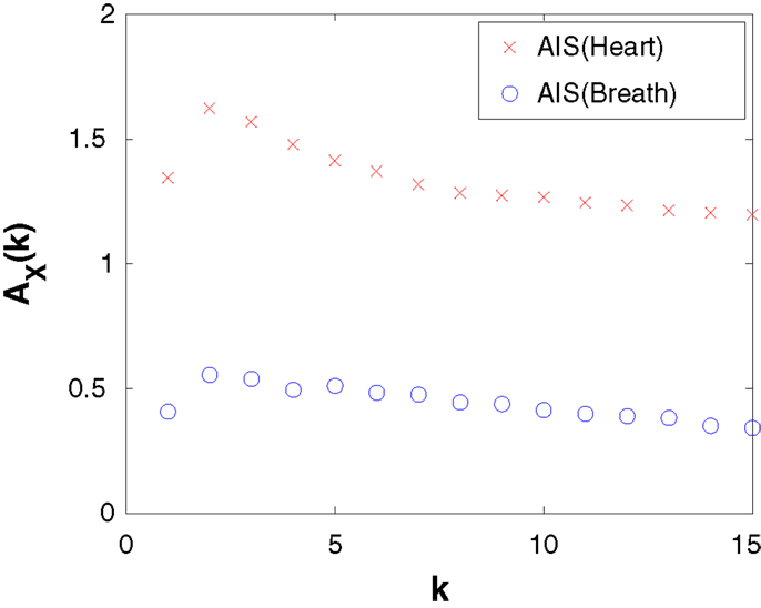
Figure 3. Active information storage (AIS) computed by the KSG estimator (K = 4 nearest neighbors) as a function of embedded history length k for the heart and breath rate time-series data.

4.5. Cellular Automata Demos

The “Cellular Automata Demos” set at demos/octave/CellularAutomata in the distribution provide a standalone demonstration of the utility of local information dynamics profiles. The scripts allow the user to reproduce the key results from Lizier et al. (2008c, 2010, 2012b, 2014); (Lizier, 2013); (Lizier and Mahoney, 2013), etc., i.e., plotting local information dynamics measures at every point in space-time in the cellular automata (CA). These results confirmed the long-held conjectures that gliders are the dominant information transfer entities in CAs, while blinkers and background domains are the dominant information storage components, and glider/particle collisions are the dominant information modification events.

The set is described in some detail at the CellularAutomataDemos wiki page (see Table 2). The demo can be run in MATLAB or Octave. The main file for the demo is plotLocalInfoMeasureForCA.m, which can be used to specify a CA type to run and which measure to plot an information profile for. Several higher-level scripts are available to demonstrate how to call this, including DirectedMeasuresChapterDemo2013.m which was used to generate the figures by Lizier (2014) (reproduced in Figure 4).

FIGURE 4

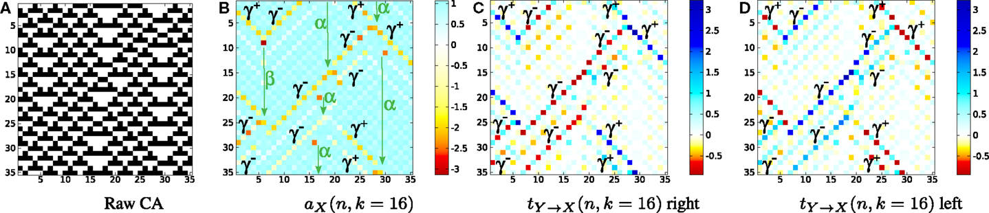
Figure 4. Local information dynamics in ECA rule 54 for the raw values in (A) (black for “1,” white for “0”). Thirty-five time steps are displayed for 35 cells, and time increases down the page for all CA plots. All units are in bits, as per scales on the right-hand sides. (B) Local active information storage; local apparent transfer entropy: (C) one cell to the right, and (D) one cell to the left per time step. NB: Reprinted with kind permission of Springer Science + Business Media from Lizier (2014).

4.6. Other Demos

The toolkit contains a number of other demonstrations, which we briefly mention here:

• The “Interregional Transfer demo” set at demos/java/interregionalTransfer/is a higher-level example of computing information transfer between two regions of variables (e.g., brain regions in fMRI data), using multivariate extensions to the transfer entropy, to infer effective connections between the regions. This demonstration implements the method originally described by Lizier et al. (2011a). Further documentation is provided via the Demos wiki page (see Table 2).

• The “Detecting interaction lags” demo set at demos/octave/DetectingInteractionLags shows how to use the transfer entropy calculators to investigate a source-destination lag that is different to 1 (the default). In particular, this demo was used to make the comparisons of using transfer entropy (TE) and momentary information transfer (MIT) (Pompe and Runge, 2011) to investigate source-destination lags by Wibral et al. (2013) (see Test cases Ia and Ib therein). In particular, the results show that TE is most suitable for investigating source-destination lags as MIT can be deceived by source memory, and also that symbolic TE (Section S.2.2.4 in Supplementary Material) can miss important components of information in an interaction. Further documentation is provided via the Demos wiki page (see Table 2).

• The “Null distribution” demo set at demos/octave/NullDistributions explores the match between analytic and resampled distributions of MI, conditional MI and TE under null hypotheses of no relationship between the data sets (see Section S.1.5 in Supplementary Material). Further documentation is provided via the Demos wiki page (see Table 2).

Finally, we note that demonstrations on using JIDT within several additional languages (Julia, Clojure, and R) are currently available within the SVN repository only, and will be distributed in future releases.

5. Conclusion

We have described the Java Information Dynamics Toolkit (JIDT), an open-source toolkit available on Google code, which implements information-theoretic measures of dynamics via several different estimators. We have described the architecture behind the toolkit and how to use it, providing several detailed code demonstrations.

In comparison to related toolkits, JIDT provides implementations for a wider array of information-theoretic measures, with a wider variety of estimators implemented, adds implementations of local measures and statistical significance, and is standalone software. Furthermore, being implemented in Java, JIDT is platform agnostic and requires little to no installation, is fast, exhibits an intuitive object-oriented design, and can be used in MATLAB, Octave, Python, and other environments.

JIDT has been used to produce results in publications by both this author and others (Wang et al., 2012, 2014; Dasgupta et al., 2013; Lizier and Mahoney, 2013; Wibral et al., 2013, 2014a,c; Gómez et al., 2014; Lizier, 2014; Lizier et al., 2014).

It may be complemented by the Java Partial Information Decomposition (JPID) toolkit (Lizier and Flecker, 2012; Lizier et al., 2013), which implements early attempts (Williams and Beer, 2010b) to separately measure redundant and synergistic components of the conditional mutual information (see Section S.1.1 in Supplementary Material).

We are planning the extension or addition of several important components in the future. Of highest priority, we are exploring the use of multi-threading and GPU computing, and automated parameter selection for time-series embedding. We will add additional implementations to complete Table 3, and aim for larger code coverage by our unit tests. Most importantly, however, we seek collaboration on the project from other developers in order to expand the capabilities of JIDT, and we will welcome volunteers who wish to contribute to the project.

Conflict of Interest Statement

The Review Editor Keyan Ghazi-Zahedi declares that, despite being affiliated to the same institution as author Joseph T. Lizier, the review process was handled objectively and no conflict of interest exists. The author declares that the research was conducted in the absence of any commercial or financial relationships that could be construed as a potential conflict of interest.

Acknowledgments

I am grateful to many collaborators and contacts who have tested JIDT in their applications, provided test data, found bugs, provided feedback, and reviewed this manuscript, etc. These include primarily X. Rosalind Wang, Michael Wibral, Oliver Cliff, Siddharth Pritam, Rommel Ceguerra, Ipek Özdemir, and Oliver Obst; as well as Sakyasingha Dasgupta, Heni Ben Amor, Mizuki Oka, Christoph Hartmann, Michael Harré, and Patricia Wollstadt.

Supplementary Material

The Supplementary Material for this article can be found online at http://www.frontiersin.org/Journal/10.3389/frobt.2014.00011/abstract

Footnotes

1. ^Further commentary on links between information-theoretic analysis and traditional dynamical systems approaches are discussed by Beer and Williams (2014).
2. ^We use the corresponding notation $X_{n+1}^{\left(k+\right)}$ for the next k values from n + 1 onwards, {X_n+1, X_n+2, …, X_n+k}, with realizations $x_{n+1}^{\left(k+\right)}=\left\{x_{n+1},x_{n+2},\dots ,x_{n+k}\right\}$
3. ^We can use an embedding delay τ to give $x_n^{\left(k\right)}=\left\{x_{n-\left(k-1\right)\mathrm{\tau }},\dots ,x_{n-\mathrm{\tau }},x_n\right\},$ where this helps to better empirically capture the state from a finite sample size. Non-uniform embeddings (i.e., with irregular delays) may also be useful (Faes et al., 2011) (not implemented in JIDT at this stage).
4. ^Except where otherwise noted, JIDT implements the most efficient described algorithm for each estimator.
5. ^http://www.trentool.de
6. ^http://figshare.com/articles/MuTE_toolbox_to_evaluate_Multivariate_Transfer_Entropy/1005245/1
7. ^http://code.google.com/p/transfer-entropy-toolbox/
8. ^http://www.ucl.ac.uk/ion/departments/sobell/Research/RLemon/MILCA/MILCA
9. ^http://www.cs.tut.fi/%7etimhome/tim/tim.htm
10. ^http://www.sussex.ac.uk/sackler/mvgc/
11. ^http://code.google.com/p/information-dynamics-toolkit/
12. ^The JIDT v1.0 distribution is compiled by Java Standard Edition 6; it is also verified as compatible with Edition 7.
13. ^http://commons.apache.org/proper/commons-math/
14. ^http://math.nist.gov/javanumerics/jama/
15. ^http://octave.sourceforge.net/java/
16. ^This is also the case for the measures for discrete data, though to a lesser degree and without multiple estimator types, so this is not focused on here.
17. ^Abstract classes provide implementations of some but not all methods required for a class, so they cannot be directly instantiated themselves but child classes, which provide implementations for the missing methods and may be instantiated.
18. ^http://www.junit.org/
19. ^The batch files are not included in release v1.0, but are currently available via the SVN repository and will be distributed in future releases.
20. ^The return format is more complicated if the user has supplied observations via several addObservations() calls rather than setObservations(); see the Javadocs for computeLocalOfPreviousObservations() for details.
21. ^In fact, for MI, JIDT does not actually define a separate calculator for univariates – the multivariate calculator MutualInfoCalculatorMultiVariate provides interfaces to supply univariate double[] data where each variable is univariate.
22. ^http://jpype.sourceforge.net/
23. ^This data set was made available via the Santa Fe Institute time series contest held in 1991 (Rigney et al., 1993) and redistributed with JIDT with kind permission from Andreas Weigend.

References

Adami, C. (2002). What is complexity? Bioessays 24, 1085–1094. doi: 10.1002/bies.10192

CrossRef Full Text | Google Scholar

Ash, R. B. (1965). Information Theory. New York, NY: Dover Publications Inc.

Google Scholar

Astakhov, S., Grassberger, P., Kraskov, A., and Stögbauer, H. (2013). Mutual Information Least-Dependent Component Analysis (MILCA). Available from: http://www.ucl.ac.uk/ion/departments/sobell/Research/RLemon/MILCA/MILCA

Google Scholar

Ay, N., Bertschinger, N., Der, R., Güttler, F., and Olbrich, E. (2008). Predictive information and explorative behavior of autonomous robots. Eur. Phys. J. B 63, 329–339. doi:10.1140/epjb/e2008-00175-0

CrossRef Full Text | Google Scholar

Bandt, C., and Pompe, B. (2002). Permutation entropy: a natural complexity measure for time series. Phys. Rev. Lett. 88, 174102. doi:10.1103/PhysRevLett.88.174102

Pubmed Abstract | Pubmed Full Text | CrossRef Full Text | Google Scholar

Barnett, L., Barrett, A. B., and Seth, A. K. (2009). Granger causality and transfer entropy are equivalent for Gaussian variables. Phys. Rev. Lett. 103, 238701. doi:10.1103/PhysRevLett.103.238701

Pubmed Abstract | Pubmed Full Text | CrossRef Full Text | Google Scholar

Barnett, L., and Bossomaier, T. (2012). Transfer entropy as a log-likelihood ratio. Phys. Rev. Lett. 109, 138105. doi:10.1103/PhysRevLett.109.138105

Pubmed Abstract | Pubmed Full Text | CrossRef Full Text | Google Scholar

Barnett, L., Lizier, J. T., Harré, M., Seth, A. K., and Bossomaier, T. (2013). Information flow in a kinetic Ising model peaks in the disordered phase. Phys. Rev. Lett. 111, 177203. doi:10.1103/PhysRevLett.111.177203

Pubmed Abstract | Pubmed Full Text | CrossRef Full Text | Google Scholar

Barnett, L., and Seth, A. K. (2014). The MVGC multivariate granger causality toolbox: a new approach to granger-causal inference. J. Neurosci. Methods 223, 50–68. doi:10.1016/j.jneumeth.2013.10.018

Pubmed Abstract | Pubmed Full Text | CrossRef Full Text | Google Scholar

Bauer, T. L., Colbaugh, R., Glass, K., and Schnizlein, D. (2013). “Use of transfer entropy to infer relationships from behavior,” in Proceedings of the Eighth Annual Cyber Security and Information Intelligence Research Workshop, CSIIRW’13 (New York, NY: ACM). doi:10.1145/2459976.2460016

CrossRef Full Text | Google Scholar

Beer, R. D., and Williams, P. L. (2014). Information processing and dynamics in minimally cognitive agents. Cogn. Sci. doi:10.1111/cogs.12142

Pubmed Abstract | Pubmed Full Text | CrossRef Full Text | Google Scholar

Bialek, W., Nemenman, I., and Tishby, N. (2001). Complexity through non-extensivity. Physica A 302, 89–99. doi:10.1186/1752-0509-5-61

Pubmed Abstract | Pubmed Full Text | CrossRef Full Text | Google Scholar

Boedecker, J., Obst, O., Lizier, J. T., Mayer, N. M., and Asada, M. (2012). Information processing in echo state networks at the edge of chaos. Theory Biosci. 131, 205–213. doi:10.1007/s12064-011-0146-8

Pubmed Abstract | Pubmed Full Text | CrossRef Full Text | Google Scholar

Bonachela, J. A., Hinrichsen, H., and Muñoz, M. A. (2008). Entropy estimates of small data sets. J. Phys. A Math. Theor. 41, 202001. doi:10.1088/1751-8113/41/20/202001

CrossRef Full Text | Google Scholar

Chávez, M., Martinerie, J., and LeVanQuyen, M. (2003). Statistical assessment of non-linear causality: application to epileptic EEG signals. J. Neurosci. Methods 124, 113–128. doi:10.1016/S0165-0270(02)00367-9

CrossRef Full Text | Google Scholar

Cliff, O. M., Lizier, J. T., Wang, X. R., Wang, P., Obst, O., and Prokopenko, M. (2014). “Towards quantifying interaction networks in a football match,” in RoboCup 2013: Robot World Cup XVII, Volume 8371 of Lecture Notes in Computer Science, eds S. Behnke, M. Veloso, A. Visser, and R. Xiong (Berlin: Springer), 1–12.

Google Scholar

Computer Language Benchmarks Game. (2014). Available at: http://benchmarksgame.alioth.debian.org/u64q/java.php

Google Scholar

Cover, T. M., and Thomas, J. A. (1991). Elements of Information Theory (Wiley Series in Telecommunications and Signal Processing). New York, NY: Wiley-Interscience.

Google Scholar

Crutchfield, J. P., and Feldman, D. P. (2003). Regularities unseen, randomness observed: levels of entropy convergence. Chaos 13, 25–54. doi:10.1063/1.1530990

Pubmed Abstract | Pubmed Full Text | CrossRef Full Text | Google Scholar

Damiani, C., Kauffman, S., Serra, R., Villani, M., and Colacci, A. (2010). “Information transfer among coupled random Boolean networks,” in Cellular Automata, Volume 6350 of Lecture Notes in Computer Science, eds S. Bandini, S. Manzoni, H. Umeo, and G. Vizzari (Berlin: Springer), 1–11.

Google Scholar

Damiani, C., and Lecca, P. (2011). “Model identification using correlation-based inference and transfer entropy estimation,” in Fifth UKSim European Symposium on Computer Modeling and Simulation (EMS) (Madrid: IEEE), 129–134.

Google Scholar

Dasgupta, S., Wörgötter, F., and Manoonpong, P. (2013). Information dynamics based self-adaptive reservoir for delay temporal memory tasks. Evolving Systems 4, 235–249. doi:10.1007/s12530-013-9080-y

CrossRef Full Text | Google Scholar

Faes, L., Nollo, G., and Porta, A. (2011). Information-based detection of non-linear granger causality in multivariate processes via a non-uniform embedding technique. Phys. Rev. E 83, 051112. doi:10.1103/PhysRevE.83.051112

Pubmed Abstract | Pubmed Full Text | CrossRef Full Text | Google Scholar

Faes, L., and Porta, A. (2014). “Conditional entropy-based evaluation of information dynamics in physiological systems,” in Directed Information Measures in Neuroscience, Understanding Complex Systems, eds M. Wibral, R. Vicente, and J. T. Lizier (Berlin: Springer), 61–86.

Google Scholar

Fano, R. M. (1961). Transmission of Information: A Statistical Theory of Communications. Cambridge, MA: MIT Press.

Google Scholar

Fernández, P., and Solé, R. V. (2006). “The role of computation in complex regulatory networks,” in Power Laws, Scale-Free Networks and Genome Biology, Molecular Biology Intelligence Unit, eds E. V. Koonin, Y. I. Wolf, and G. P. Karev (Springer), 206–225. doi:10.1007/0-387-33916-7_12

CrossRef Full Text | Google Scholar

Frenzel, S., and Pompe, B. (2007). Partial mutual information for coupling analysis of multivariate time series. Phys. Rev. Lett. 99, 204101. doi:10.1103/PhysRevLett.99.204101

Pubmed Abstract | Pubmed Full Text | CrossRef Full Text | Google Scholar

Gell-Mann, M. (1994). The Quark and the Jaguar. New York, NY: W.H. Freeman.

Google Scholar

Gómez, C., Lizier, J. T., Schaum, M., Wollstadt, P., Grützner, C., Uhlhaas, P., et al. (2014). Reduced predictable information in brain signals in autism spectrum disorder. Front. Neuroinformatics 8:9. doi:10.3389/fninf.2014.00009

Pubmed Abstract | Pubmed Full Text | CrossRef Full Text | Google Scholar

Gomez-Herrero, G., Wu, W., Rutanen, K., Soriano, M. C., Pipa, G., and Vicente, R. (2010). Assessing coupling dynamics from an ensemble of time series. arXiv:1008.0539.

Google Scholar

Gong, P., and van Leeuwen, C. (2009). Distributed dynamical computation in neural circuits with propagating coherent activity patterns. PLoS Comput. Biol. 5:e1000611. doi:10.1371/journal.pcbi.1000611

Pubmed Abstract | Pubmed Full Text | CrossRef Full Text | Google Scholar

Grassberger, P. (1986). Toward a quantitative theory of self-generated complexity. Int. J. Theor. Phys. 25, 907–938. doi:10.1007/BF00668821

CrossRef Full Text | Google Scholar

Helvik, T., Lindgren, K., and Nordahl, M. G. (2004). “Local information in one-dimensional cellular automata,” in Proceedings of the International Conference on Cellular Automata for Research and Industry, Amsterdam, Volume 3305 of Lecture Notes in Computer Science, eds P. M. A. Sloot, B. Chopard, and A. G. Hoekstra (Berlin: Springer), 121–130.

Google Scholar

Honey, C. J., Kötter, R., Breakspear, M., and Sporns, O. (2007). Network structure of cerebral cortex shapes functional connectivity on multiple time scales. Proc. Natl. Acad. Sci. U.S.A. 104, 10240–10245. doi:10.1073/pnas.0701519104

Pubmed Abstract | Pubmed Full Text | CrossRef Full Text | Google Scholar

Ito, S., Hansen, M. E., Heiland, R., Lumsdaine, A., Litke, A. M., and Beggs, J. M. (2011). Extending transfer entropy improves identification of effective connectivity in a spiking cortical network model. PLoS ONE 6:e27431. doi:10.1371/journal.pone.0027431

Pubmed Abstract | Pubmed Full Text | CrossRef Full Text | Google Scholar

Kaiser, A., and Schreiber, T. (2002). Information transfer in continuous processes. Physica D 166, 43–62. doi:10.1016/S0167-2789(02)00432-3

CrossRef Full Text | Google Scholar

Kantz, H., and Schreiber, T. (1997). Non-Linear Time Series Analysis. Cambridge, MA: Cambridge University Press.

Google Scholar

Klyubin, A. S., Polani, D., and Nehaniv, C. L. (2008). Keep your options open: an information-based driving principle for sensorimotor systems. PLoS ONE 3:e4018. doi:10.1371/journal.pone.0004018

Pubmed Abstract | Pubmed Full Text | CrossRef Full Text | Google Scholar

Kozachenko, L., and Leonenko, N. (1987). A statistical estimate for the entropy of a random vector. Probl. Inf. Transm. 23, 9–16.

Pubmed Abstract | Pubmed Full Text | Google Scholar

Kraskov, A., Stögbauer, H., and Grassberger, P. (2004). Estimating mutual information. Phys. Rev. E 69, 066138. doi:10.1103/PhysRevE.69.066138

Pubmed Abstract | Pubmed Full Text | CrossRef Full Text | Google Scholar

Langton, C. G. (1990). Computation at the edge of chaos: phase transitions and emergent computation. Physica D 42, 12–37. doi:10.1016/0167-2789(90)90064-V

CrossRef Full Text | Google Scholar

Liao, W., Ding, J., Marinazzo, D., Xu, Q., Wang, Z., Yuan, C., et al. (2011). Small-world directed networks in the human brain: multivariate granger causality analysis of resting-state fMRI. Neuroimage 54, 2683–2694. doi:10.1016/j.neuroimage.2010.11.007

Pubmed Abstract | Pubmed Full Text | CrossRef Full Text | Google Scholar

Lindner, M., Vicente, R., Priesemann, V., and Wibral, M. (2011). TRENTOOL: a MATLAB open source toolbox to analyse information flow in time series data with transfer entropy. BMC Neurosci. 12:119. doi:10.1186/1471-2202-12-119

Pubmed Abstract | Pubmed Full Text | CrossRef Full Text | Google Scholar

Lizier, J. T. (2013). The Local Information Dynamics of Distributed Computation in Complex Systems (Springer Theses). Berlin: Springer.

Google Scholar

Lizier, J. T. (2014). “Measuring the dynamics of information processing on a local scale in time and space,” in Directed Information Measures in Neuroscience, Understanding Complex Systems, eds M. Wibral, R. Vicente, and J. T. Lizier (Berlin: Springer), 161–193.

Google Scholar

Lizier, J. T., Atay, F. M., and Jost, J. (2012a). Information storage, loop motifs, and clustered structure in complex networks. Phys. Rev. E 86, 026110. doi:10.1103/PhysRevE.86.026110

Pubmed Abstract | Pubmed Full Text | CrossRef Full Text | Google Scholar

Lizier, J. T., Prokopenko, M., and Zomaya, A. Y. (2012b). Local measures of information storage in complex distributed computation. Inf. Sci. 208, 39–54. doi:10.1016/j.ins.2012.04.016

CrossRef Full Text | Google Scholar

Lizier, J. T., and Flecker, B. (2012). Java Partial Information Decomposition Toolkit. Available at: http://github.com/jlizier/jpid

Google Scholar

Lizier, J. T., Flecker, B., and Williams, P. L. (2013). “Towards a synergy-based approach to measuring information modification,” in Proceedings of the 2013 IEEE Symposium on Artificial Life (ALIFE) (Singapore: IEEE), 43–51.

Google Scholar

Lizier, J. T., Heinzle, J., Horstmann, A., Haynes, J.-D., and Prokopenko, M. (2011a). Multivariate information-theoretic measures reveal directed information structure and task relevant changes in fMRI connectivity. J. Comput. Neurosci. 30, 85–107. doi:10.1007/s10827-010-0271-2

Pubmed Abstract | Pubmed Full Text | CrossRef Full Text | Google Scholar

Lizier, J. T., Piraveenan, M., Pradhana, D., Prokopenko, M., and Yaeger, L. S. (2011b). “Functional and structural topologies in evolved neural networks,” in Proceedings of the European Conference on Artificial Life (ECAL), Volume 5777 of Lecture Notes in Computer Science, eds G. Kampis, I. Karsai, and E. Szathmáry (Berlin: Springer), 140–147.

Google Scholar

Lizier, J. T., Pritam, S., and Prokopenko, M. (2011c). Information dynamics in small-world Boolean networks. Artif. Life 17, 293–314. doi:10.1162/artl_a_00040

Pubmed Abstract | Pubmed Full Text | CrossRef Full Text | Google Scholar

Lizier, J. T., and Mahoney, J. R. (2013). Moving frames of reference, relativity and invariance in transfer entropy and information dynamics. Entropy 15, 177–197. doi:10.3390/e15010177

CrossRef Full Text | Google Scholar

Lizier, J. T., Prokopenko, M., Tanev, I., and Zomaya, A. Y. (2008a). “Emergence of glider-like structures in a modular robotic system,” in Proceedings of the Eleventh International Conference on the Simulation and Synthesis of Living Systems (ALife XI), Winchester, UK, eds S. Bullock, J. Noble, R. Watson, and M. A. Bedau (Cambridge, MA: MIT Press), 366–373.

Google Scholar

Lizier, J. T., Prokopenko, M., and Zomaya, A. Y. (2008b). “The information dynamics of phase transitions in random Boolean networks,” in Proceedings of the Eleventh International Conference on the Simulation and Synthesis of Living Systems (ALife XI), Winchester, UK, eds S. Bullock, J. Noble, R. Watson, and M. A. Bedau (Cambridge, MA: MIT Press), 374–381.

Google Scholar

Lizier, J. T., Prokopenko, M., and Zomaya, A. Y. (2008c). Local information transfer as a spatiotemporal filter for complex systems. Phys. Rev. E 77, 026110. doi:10.1103/PhysRevE.77.026110

Pubmed Abstract | Pubmed Full Text | CrossRef Full Text | Google Scholar

Lizier, J. T., Prokopenko, M., and Zomaya, A. Y. (2007). “Detecting non-trivial computation in complex dynamics,” in Proceedings of the 9th European Conference on Artificial Life (ECAL 2007), Volume 4648 of Lecture Notes in Computer Science, eds F. Almeida e Costa, L. M. Rocha, E. Costa, I. Harvey, and A. Coutinho (Berlin: Springer), 895–904.

Google Scholar

Lizier, J. T., Prokopenko, M., and Zomaya, A. Y. (2010). Information modification and particle collisions in distributed computation. Chaos 20, 037109. doi:10.1063/1.3486801

Pubmed Abstract | Pubmed Full Text | CrossRef Full Text | Google Scholar

Lizier, J. T., Prokopenko, M., and Zomaya, A. Y. (2014). “A framework for the local information dynamics of distributed computation in complex systems,” in Guided Self-Organization: Inception, Volume 9 of Emergence, Complexity and Computation, ed. M. Prokopenko (Berlin: Springer), 115–158.

Google Scholar

Lungarella, M., and Sporns, O. (2006). Mapping information flow in sensorimotor networks. PLoS Comput. Biol. 2:e144. doi:10.1371/journal.pcbi.0020144

Pubmed Abstract | Pubmed Full Text | CrossRef Full Text | Google Scholar

MacKay, D. J. C. (2003). Information Theory, Inference, and Learning Algorithms. Cambridge: Cambridge University Press.

Google Scholar

Mahoney, J. R., Ellison, C. J., James, R. G., and Crutchfield, J. P. (2011). How hidden are hidden processes? A primer on crypticity and entropy convergence. Chaos 21, 037112. doi:10.1063/1.3637502

Pubmed Abstract | Pubmed Full Text | CrossRef Full Text | Google Scholar

Mäki-Marttunen, V., Diez, I., Cortes, J. M., Chialvo, D. R., and Villarreal, M. (2013). Disruption of transfer entropy and inter-hemispheric brain functional connectivity in patients with disorder of consciousness. Front. Neuroinformatics 7:24. doi:10.3389/fninf.2013.00024

Pubmed Abstract | Pubmed Full Text | CrossRef Full Text | Google Scholar

Marinazzo, D., Wu, G., Pellicoro, M., Angelini, L., and Stramaglia, S. (2012). Information flow in networks and the law of diminishing marginal returns: evidence from modeling and human electroencephalographic recordings. PLoS ONE 7:e45026. doi:10.1371/journal.pone.0045026

Pubmed Abstract | Pubmed Full Text | CrossRef Full Text | Google Scholar

Miramontes, O. (1995). Order-disorder transitions in the behavior of ant societies. Complexity 1, 56–60. doi:10.1002/cplx.6130010313

CrossRef Full Text | Google Scholar

Mitchell, M. (1998). “Computation in cellular automata: a selected review,” in Non-Standard Computation, eds T. Gramß, S. Bornholdt, M. Groß, M. Mitchell, and T. Pellizzari (Weinheim: Wiley-VCH Verlag GmbH & Co. KGaA), 95–140.

Google Scholar

Mitchell, M. (2009). Complexity: A Guided Tour. New York, NY: Oxford University Press.

Google Scholar

Montalto, A. (2014). MuTE Toolbox to Evaluate Multivariate Transfer Entropy. Figshare. Available at: http://dx.doi.org/10.6084/m9.figshare.1005245

Google Scholar

Montalto, A., Faes, L., and Marinazzo, D. (2014a). MuTE: a MATLAB toolbox to compare established and novel estimators of the multivariate transfer entropy. PLoS ONE 9:e109462. doi:10.1371/journal.pone.0109462

Pubmed Abstract | Pubmed Full Text | CrossRef Full Text | Google Scholar

Montalto, A., Faes, L., and Marinazzo, D. (2014b). “MuTE: a new MATLAB toolbox for estimating the multivariate transfer entropy in physiological variability series,” in 8th Conference of the European Study Group on Cardiovascular Oscillations (ESGCO) (Trento: IEEE), 59–60. doi:10.1109/ESGCO.2014.6847518

CrossRef Full Text | Google Scholar

Nakajima, K., and Haruna, T. (2013). Symbolic local information transfer. Eur. Phys. J. Spec. Top. 222, 437–455. doi:10.1140/epjst/e2013-01851-x

CrossRef Full Text | Google Scholar

Nakajima, K., Li, T., Kang, R., Guglielmino, E., Caldwell, D. G., and Pfeifer, R. (2012). “Local information transfer in soft robotic arm,” in IEEE International Conference on Robotics and Biomimetics (ROBIO) (Guangzhou: IEEE), 1273–1280.

Google Scholar

Nilsson, M., and Kleijn, W. B. (2007). On the estimation of differential entropy from data located on embedded manifolds. IEEE Trans. Inf. Theory 53, 2330–2341. doi:10.1109/TIT.2007.899533

CrossRef Full Text | Google Scholar

Obst, O., Boedecker, J., and Asada, M. (2010). “Improving recurrent neural network performance using transfer entropy neural information processing. models and applications,” in Neural Information Processing. Models and Applications, Volume 6444 of Lecture Notes in Computer Science, Chapter 24, eds K. Wong, B. Mendis, and A. Bouzerdoum (Berlin: Springer), 193–200.

Google Scholar

Obst, O., Boedecker, J., Schmidt, B., and Asada, M. (2013). On active information storage in input-driven systems. arXiv:1303.5526.

Google Scholar

Oka, M., and Ikegami, T. (2013). Exploring default mode and information flow on the web. PLoS ONE 8:e60398. doi:10.1371/journal.pone.0060398

Pubmed Abstract | Pubmed Full Text | CrossRef Full Text | Google Scholar

Oostenveld, R., Fries, P., Maris, E., and Schoffelen, J.-M. (2011). FieldTrip: open source software for advanced analysis of MEG, EEG, and invasive electrophysiological data. Comput. Intell. Neurosci. 2011, 156869. doi:10.1155/2011/156869

Pubmed Abstract | Pubmed Full Text | CrossRef Full Text | Google Scholar

Orlandi, J., Saeed, M., and Guyon, I. (2014). Chalearn Connectomics Challenge Sample Code. Available at: http://connectomics.chalearn.org

Google Scholar

Paninski, L. (2003). Estimation of entropy and mutual information. Neural Comput. 15, 1191–1253. doi:10.1162/089976603321780272

CrossRef Full Text | Google Scholar

Piraveenan, M., Prokopenko, M., and Zomaya, A. Y. (2009). Assortativeness and information in scale-free networks. Eur. Phys. J. B 67, 291–300. doi:10.1140/epjb/e2008-00473-5

CrossRef Full Text | Google Scholar

Pompe, B., and Runge, J. (2011). Momentary information transfer as a coupling measure of time series. Phys. Rev. E 83, 051122. doi:10.1103/PhysRevE.83.051122

Pubmed Abstract | Pubmed Full Text | CrossRef Full Text | Google Scholar

Prokopenko, M. (2009). Guided self-organization. HFSP J. 3, 287–289. doi:10.2976/1.3233933

CrossRef Full Text | Google Scholar

Prokopenko, M., Boschietti, F., and Ryan, A. J. (2009). An information-theoretic primer on complexity, self-organization, and emergence. Complexity 15, 11–28. doi:10.1002/cplx.20249

CrossRef Full Text | Google Scholar

Prokopenko, M., Gerasimov, V., and Tanev, I. (2006a). “Evolving spatiotemporal coordination in a modular robotic system,” in From Animals to Animats 9: Proceedings of the Ninth International Conference on the Simulation of Adaptive Behavior (SAB’06), Volume 4095 of Lecture Notes in Computer Science, eds S. Nolfi, G. Baldassarre, R. Calabretta, J. C. T. Hallam, D. Marocco, J.-A. Meyer, (Berlin: Springer), 558–569.

Google Scholar

Prokopenko, M., Gerasimov, V., and Tanev, I. (2006b). “Measuring spatiotemporal coordination in a modular robotic system,” in Proceedings of the 10th International Conference on the Simulation and Synthesis of Living Systems (ALifeX), Bloomington, Indiana, USA, eds L. M. Rocha, L. S. Yaeger, M. A. Bedau, D. Floreano, R. L. Goldstone, and A. Vespignani (Bloomington: MIT Press), 185–191.

Google Scholar

Prokopenko, M., Lizier, J. T., Obst, O., and Wang, X. R. (2011). Relating Fisher information to order parameters. Phys. Rev. E 84, 041116. doi:10.1103/PhysRevE.84.041116

Pubmed Abstract | Pubmed Full Text | CrossRef Full Text | Google Scholar

Prokopenko, M., Wang, P., Valencia, P., Price, D., Foreman, M., and Farmer, A. (2005). Self-organizing hierarchies in sensor and communication networks. Artif. Life 11, 407–426. doi:10.1162/106454605774270642

Pubmed Abstract | Pubmed Full Text | CrossRef Full Text | Google Scholar

Rigney, D. R., Goldberger, A. L., Ocasio, W., Ichimaru, Y., Moody, G. B., and Mark, R. (1993). “Multi-channel physiological data: description and analysis,” in Time Series Prediction: Forecasting the Future and Understanding the Past, eds A. S. Weigend and N. A. Gershenfeld (Reading, MA: Addison-Wesley), 105–129.

Google Scholar

Rutanen, K. (2011). Tim 1.2.0. Available at: http://www.cs.tut.fi/~timhome/tim-1.2.0/tim.htm

Google Scholar

Sandoval, L. (2014). Structure of a global network of financial companies based on transfer entropy. Entropy 16, 4443–4482. doi:10.3390/e16084443

CrossRef Full Text | Google Scholar

Schreiber, T. (2000). Measuring information transfer. Phys. Rev. Lett. 85, 461–464. doi:10.1103/PhysRevLett.85.461

Pubmed Abstract | Pubmed Full Text | CrossRef Full Text | Google Scholar

Shalizi, C. R., Haslinger, R., Rouquier, J.-B., Klinkner, K. L., and Moore, C. (2006). Automatic filters for the detection of coherent structure in spatiotemporal systems. Phys. Rev. E 73, 036104. doi:10.1103/PhysRevE.73.036104

Pubmed Abstract | Pubmed Full Text | CrossRef Full Text | Google Scholar

Shalizi, C. R. (2001). Causal Architecture, Complexity and Self-Organization in Time Series and Cellular Automata. Ph.D., thesis, University of Wisconsin-Madison, Madison, WI.

Google Scholar

Shannon, C. E. (1948). A mathematical theory of communication. Bell Syst. Tech. J. 27, 379–423. doi:10.1002/j.1538-7305.1948.tb01338.x

CrossRef Full Text | Google Scholar

Solé, R. V., and Valverde, S. (2001). Information transfer and phase transitions in a model of internet traffic. Physica A 289, 595–605. doi:10.1016/S0378-4371(00)00536-7

CrossRef Full Text | Google Scholar

Solé, R. V., and Valverde, S. (2004). “Information theory of complex networks: on evolution and architectural constraints,” in Complex Networks, Volume 650 of Lecture Notes in Physics, eds E. Ben-Naim, H. Frauenfelder, and Z. Toroczkai (Berlin: Springer), 189–207.

Google Scholar

Staniek, M., and Lehnertz, K. (2008). Symbolic transfer entropy. Phys. Rev. Lett. 100, 158101. doi:10.1103/PhysRevLett.100.158101

Pubmed Abstract | Pubmed Full Text | CrossRef Full Text | Google Scholar

Steeg, G. V., and Galstyan, A. (2013). “Information-theoretic measures of influence based on content dynamics,” in Proceedings of the Sixth ACM International Conference on Web Search and Data Mining, WSDM’13 (New York, NY: ACM), 3–12.

Google Scholar

Stetter, O., Battaglia, D., Soriano, J., and Geisel, T. (2012). Model-free reconstruction of excitatory neuronal connectivity from calcium imaging signals. PLoS Comput. Biol. 8:e1002653. doi:10.1371/journal.pcbi.1002653

Pubmed Abstract | Pubmed Full Text | CrossRef Full Text | Google Scholar

Stögbauer, H., Kraskov, A., Astakhov, S., and Grassberger, P. (2004). Least-dependent-component analysis based on mutual information. Phys. Rev. E 70, 066123. doi:10.1103/PhysRevE.70.066123

Pubmed Abstract | Pubmed Full Text | CrossRef Full Text | Google Scholar

Stowell, D., and Plumbley, M. D. (2009). Fast multidimensional entropy estimation by k-d partitioning. IEEE Signal Process. Lett. 16, 537–540. doi:10.1109/LSP.2009.2017346

CrossRef Full Text | Google Scholar

Stramaglia, S., Wu, G.-R., Pellicoro, M., and Marinazzo, D. (2012). “Expanding the transfer entropy to identify information subgraphs in complex systems,” in Annual International Conference of the IEEE Engineering in Medicine and Biology Society (San Diego, CA: IEEE), 3668–3671.

Google Scholar

Takens, F. (1981). “Detecting strange attractors in turbulence,” in Dynamical Systems and Turbulence, Warwick 1980, Volume 898 of Lecture Notes in Mathematics, Chapter 21, eds D. Rand and L.-S. Young (Berlin: Springer), 366–381.

Google Scholar

Tononi, G., Sporns, O., and Edelman, G. M. (1994). A measure for brain complexity: relating functional segregation and integration in the nervous system. Proc. Natl. Acad. Sci. U.S.A. 91, 5033–5037. doi:10.1073/pnas.91.11.5033

Pubmed Abstract | Pubmed Full Text | CrossRef Full Text | Google Scholar

Vakorin, V. A., Krakovska, O. A., and McIntosh, A. R. (2009). Confounding effects of indirect connections on causality estimation. J. Neurosci. Methods 184, 152–160. doi:10.1016/j.jneumeth.2009.07.014

Pubmed Abstract | Pubmed Full Text | CrossRef Full Text | Google Scholar

Verdes, P. F. (2005). Assessing causality from multivariate time series. Phys. Rev. E 72, 026222. doi:10.1103/PhysRevE.72.026222

Pubmed Abstract | Pubmed Full Text | CrossRef Full Text | Google Scholar

Vicente, R., and Wibral, M. (2014). “Efficient estimation of information transfer,” in Directed Information Measures in Neuroscience, Understanding Complex Systems, eds M. Wibral, R. Vicente, and J. T. Lizier (Berlin: Springer), 37–58.

Google Scholar

Vicente, R., Wibral, M., Lindner, M., and Pipa, G. (2011). Transfer entropy – a model-free measure of effective connectivity for the neurosciences. J. Comput. Neurosci. 30, 45–67. doi:10.1007/s10827-010-0262-3

Pubmed Abstract | Pubmed Full Text | CrossRef Full Text | Google Scholar

Walker, S. I., Cisneros, L., and Davies, P. C. W. (2012). “Evolutionary transitions and top-down causation,” in Artificial Life 13 (East Lansing, MI: MIT Press), 283–290.

Google Scholar

Wang, X. R., Lizier, J. T., Nowotny, T., Berna, A. Z., Prokopenko, M., and Trowell, S. C. (2014). Feature selection for chemical sensor arrays using mutual information. PLoS ONE 9:e89840. doi:10.1371/journal.pone.0089840

Pubmed Abstract | Pubmed Full Text | CrossRef Full Text | Google Scholar

Wang, X. R., Miller, J. M., Lizier, J. T., Prokopenko, M., and Rossi, L. F. (2012). Quantifying and tracing information cascades in swarms. PLoS ONE 7:e40084. doi:10.1371/journal.pone.0040084

Pubmed Abstract | Pubmed Full Text | CrossRef Full Text | Google Scholar

Wibral, M., Lizier, J. T., Vögler, S., Priesemann, V., and Galuske, R. (2014a). Local active information storage as a tool to understand distributed neural information processing. Front. Neuroinformatics 8:1. doi:10.3389/fninf.2014.00001

Pubmed Abstract | Pubmed Full Text | CrossRef Full Text | Google Scholar

Wibral, M., Vicente, R., and Lindner, M. (2014b). “Transfer entropy in neuroscience,” in Directed Information Measures in Neuroscience, Understanding Complex Systems, eds M. Wibral, R. Vicente, and J. T. Lizier (Berlin: Springer), 3–36.

Google Scholar

Wibral, M., Vicente, R., and Lizier, J. T. (eds) (2014c). Directed Information Measures in Neuroscience. Berlin: Springer.

Google Scholar

Wibral, M., Pampu, N., Priesemann, V., Siebenhühner, F., Seiwert, H., Lindner, M., et al. (2013). Measuring information-transfer delays. PLoS ONE 8:e55809. doi:10.1371/journal.pone.0055809

Pubmed Abstract | Pubmed Full Text | CrossRef Full Text | Google Scholar

Wibral, M., Rahm, B., Rieder, M., Lindner, M., Vicente, R., and Kaiser, J. (2011). Transfer entropy in magnetoencephalographic data: quantifying information flow in cortical and cerebellar networks. Prog. Biophys. Mol. Biol. 105, 80–97. doi:10.1016/j.pbiomolbio.2010.11.006

Pubmed Abstract | Pubmed Full Text | CrossRef Full Text | Google Scholar

Williams, P. L., and Beer, R. D. (2010a). “Information dynamics of evolved agents,” in From Animals to Animats 11, Volume 6226 of Lecture Notes in Computer Science, Chapter 4, eds S. Doncieux, B. Girard, A. Guillot, J. Hallam, J.-A. Meyer, and J.-B. Mouret (Berlin: Springer), 38–49.

Google Scholar

Williams, P. L., and Beer, R. D. (2010b). Nonnegative decomposition of multivariate information. arXiv:1004.2515.

Pubmed Abstract | Pubmed Full Text | Google Scholar

Williams, P. L., and Beer, R. D. (2011). Generalized measures of information transfer. arXiv:1102.1507.

Google Scholar

Wollstadt, P., Martínez-Zarzuela, M., Vicente, R., Díaz-Pernas, F. J., and Wibral, M. (2014). Efficient transfer entropy analysis of non-stationary neural time series. PLoS ONE 9:e102833. doi:10.1371/journal.pone.0102833

Pubmed Abstract | Pubmed Full Text | CrossRef Full Text | Google Scholar