Inferring single neuron properties in conductance based balanced networks

1 Introduction

Neurons in the cortex tend to display very irregular firing patterns. This behavior has been considered paradoxical (Softky and Koch, 1993), because if the inputs are uncorrelated or weakly correlated the central limit theorem holds and the temporal fluctuations of a large number of synaptic inputs should be much smaller than the mean. Combining this with the fact that when the neurons are stimulated with a constant input the firing is regular (Holt et al., 1996) we should obtain an approximately regular firing pattern. One explanation of the irregularity is that excitatory and inhibitory inputs could almost balance the mean values but add their fluctuations. In that way it would be possible to achieve high variability. Surprisingly, this regime can be achieved without any fine tuning of the network parameters or the intrinsic parameters of the neuron dynamics (van Vreeswijk and Sompolinsky, 1996, 1998). The only condition is that the neurons are sparsely connected with strong synapses. In the limit of infinite size and infinite number of connections (but keeping the ratio between the number of connections per neuron and the number of neurons very small), a balanced state can be achieved for a two-population network of excitatory and inhibitory neurons.

The balanced state displays some interesting features. On the one hand the input–output relation of the population activity is a linear function independently of the dynamics of the individual neurons. The input–output function of the neurons in the network, on the other hand, is strongly affected by the temporal fluctuations of the input. For binary neurons it is the convolution of the single neuron f–I curve with a Gaussian function whose variance can be evaluated self-consistently (van Vreeswijk and Sompolinsky, 1998). In general, whatever the single neuron model, the individual f–I curve of a neuron in a network will always be continuous even if the single neuron displays a discontinuous onset of firing. The temporal fluctuations of the input smooth the f–I curve in such a way that is difficult to identify the behavior of the single neuron.

In a previous work (Mato and Samengo, 2008) we used reverse correlation methods (Agüera y Arcas and Fairhall, 2003; Agüera y Arcas et al., 2003; Bialek and De Ruyter von Steveninck, 2003; Paninski, 2003; Rust et al., 2005; Hong et al., 2007; Maravall et al., 2007) to analyze the relation between the intrinsic dynamics of a neuron and the optimal stimuli that generate action potentials. In these methods a noisy input is applied to a neuron and the stimuli that precede the actions potentials are analyzed in order to extract information on the neuron dynamics. We found that Type I neurons (that undergo a saddle–node bifurcation, with a continuous f–I curve) have a depolarizing optimal stimuli, while Type II neurons (that undergo a Hopf bifurcation, with a discontinuous f–I curve; Izhikevich, 2001, 2007; Brown et al., 2004) have optimal stimuli with well defined temporal frequencies, that depend on the resonant frequencies of the model. This classification has been shown to be relevant for functional purposes. For instance in (Muresan and Savin, 2007) it has been found that networks with Type I neurons are more responsive to external inputs while networks with Type II neurons favor homeostasis and self-sustainability of the network activity. (Baroni and Varona, 2007) have suggested that the differences in the input–output transformation carried out by Type I and Type II neurons may have evolved to activate different populations of neurons, depending on the specific temporal patterns of the presynaptic input. For these reasons it is relevant to identify the neuronal type inside a network. Reverse correlation methods require a random input to a neuron. In principle this can be achieved in vitro with electrode stimulation. On the other hand, in vivo networks have a highly variable input, that in the ideal conditions of the balanced state could be used to identify the relevant features and intrinsic neuronal properties.

In this work we study the statistical properties of the synaptic input on individual neurons and on groups of neurons in order to determine if reverse correlation methods can be used without any external input. Specifically we ask: will the covariance analysis still be useful even if the input to the network is not purely Gaussian but generated by the network dynamics? Will we be able to discriminate between the different single neuron dynamics using this method? Is it possible to collect spikes from different neurons in order to shorten the total time that is needed for the simulations? We analyze these questions under reasonably realistic conditions for the synaptic time constants and strength of the synaptic interactions.

The paper is organized as follows. In the Section 2 we introduce the network architecture and we review the properties of the balanced state and the covariance analysis for extracting the relevant features. In the Section 3 we show examples of Type I (Wang–Buszàki) and Type II networks (Hodgkin–Huxley). We also analyze “mixed” networks motivated on experimental data. The results are summarized and discussed in the last section.

2 Materials and Methods

2.1 Models of Large Networks

Our network model represents a local circuit in the cortex. It consists of N_E excitatory and N_I inhibitory conductance based neurons that represent pyramidal cells and GABAergic fast-spiking interneurons, respectively (see Figure 1). The membrane potential of neuron i in population k (k = E, I, i = 1,…, N_k,) follows the dynamics given in Section 1 in Appendix (Wang–Buszàki neurons, WB) and Section 2 in Appendix (Hodgkin–Huxley neurons, HH). The total input any neuron receives, denoted by is composed by an external input , that for simplicity is taken as the same for all the neurons in one population, and the synaptic input . The synaptic input that a neuron i in population k receives due to all its interactions with other neurons in the network is

FIGURE 1

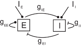
Figure 1. Diagram of the network model. Excitatory connections are represented by circles and inhibitory connections by bars.

where is the time at which neuron j in population l fires its nth action potential and the connectivity matrix of the network is: J_ik,jl = 1 if neuron (j, l) is connected pre-synaptically to neuron (i, k) and J_ik,jl = 0, otherwise. The probability of connection, between a pre-synaptic neuron (j, l) and a post-synaptic neuron (i, k; i.e., the probability that J_ik,jl = 1) depends only on the type of these neurons, i.e., P_ik,jl = P_kl = K_kl/N_l. The total number of connections that a neuron in population k receives from population l is in average K_kl. For simplicity we will take K_kl = K for all k, l.

The function f_l(t) which describes the dynamics of individual post-synaptic currents is taken to be (Koch, 1999),

where τ_l is the synaptic decay time, and Θ(t) = 0 (resp. 1) for t < 0 (resp. t ≥ 0).

In Eq. 1G_kl is the maximal efficacy of the synapses from population l to population k. In (van Vreeswijk and Sompolinsky, 1996, 1998) it is shown that the notion of balance of excitation and inhibition can be formulated rigorously in the limit of very large networks and sparse connectivity, i.e., in the limit: 1 = K = N_k, N_l. In that limit, balance of excitation and inhibition emerges naturally if the synapses are “strong” in the sense that the maximal strength of post-synaptic current, G_kl, is of the order of . This requirement implies that the total input that a neuron in population k receives from the neurons in population l is of the order of and it is therefore very large. To emphasize this requirement we parameterize the maximal synaptic efficacy as

where g_kE > 0 and g_kI < 0. Since there are in average K non-zero connections on a given neuron in population k coming from population l, the total synaptic input scales as . We also take the same scaling for the external input:

with is independent of K. In this way we have that and are proportional to .

As we will see below, it is useful to split the total input into excitatory and inhibitory components, i.e.,

where incorporates the excitatory part of the synaptic interaction and the external input and takes into account the inhibitory part of the synaptic interaction.

We shall consider three different combinations for the intrinsic dynamics of the different populations:

• Type I network: both populations (E and I) evolve according to the equations of the WB model. These neurons undergo a saddle–node bifurcation. They have a continuous f–I curve and a non-resonant behavior.

• Type II network: both populations (E and I) evolve according to the equations of the HH model. These neurons undergo a subcritical Hopf bifurcation. They have a discontinuous f–I curve and a resonant behavior generated by the spiral stability of the fixed point.

• Mixed network: 95% of the neurons in population E evolves according to the equations of the WB model and 5% according to the HH model. For the I population the proportions are the opposite (95% for HH and 5% for WB). The motivation for this choice is that it has been found that regular-spiking pyramidal neurons and fast-spiking inhibitory interneurons in layer 2/3 of somatosensory cortex tend to exhibit Type I and Type II behaviors, respectively (Tateno et al., 2004; Tateno and Robinson, 2006).

The network parameters are given in Section 3 in Appendix. Let us note that with these parameters the individual synapses have values that are in the physiological range (see for instance Reyes et al., 1998 or Rozov et al., 2001). The peak synaptic potentials (excitatory or inhibitory) go from a few tenths of mV to a few mV depending on the type of interaction (E to E, E to I, etc.), on the connectivity (the individual synapses are weaker when K is larger), and on the post-synaptic neuron dynamics.

2.2 Balanced State

According to the definitions of the previous section the total excitatory and inhibitory inputs to a given neuron can be extremely large and their value increases with the square root of the connectivity. However there is a situation where, without any fine tuning of the parameters, these inputs almost cancel each other generating a finite firing rate. This is the balanced state (van Vreeswijk and Sompolinsky, 1998). This solution can be understood in the following way. Le us suppose that the average firing rate of the excitatory (resp. inhibitory) population is given by f_E (resp. f_I). The total input on a given excitatory neuron will be approximately

Similarly for an inhibitory neuron

In the limit of infinite K the only possibility for having a finite value of the total input and therefore a finite firing rate is that

Let us note that this means that, independently of the details of the neuron dynamics, there is a linear relationship between the mean firing rate of each population and the external input. This model has been analyzed in detail in (van Vreeswijk and Sompolinsky, 2003; Lerchner et al., 2006; Hertz, 2010), showing, for instance that it leads to highly irregular firing patterns.

2.3 Extraction of Relevant Stimulus Features in a Balanced State

Here we review briefly reverse correlation methods and discuss how to apply them to networks in the balanced state. In order to explore the stimuli that are most relevant in shaping the probability of spiking, spike triggered covariance techniques have been proposed (Bialek and De Ruyter von Steveninck, 2003; Paninski, 2003; Schwartz et al., 2006). If P[spike at t₀|s(t)] is the probability to generate a spike at time t₀ conditional to a time-dependent stimulus s(t), we assume that P only depends on the noisy stimulus s(t) through a few relevant features f¹(t − t₀), f²(t − t₀),…, f^k(t − t₀). The stimulus and the relevant features are continuous functions of time. For computational purposes, however, we represent them as vectors s and fⁱ of N components, where each component s_j = s(jδt) and is the value of the stimulus evaluated at discrete intervals δt. If δt is small compared to the relevant time scales of the models this will be a good approximation.

The relevant features f¹…f^k lie in the space spanned by those eigenvectors of the matrix whose eigenvalues are significantly different from unity (Schwartz et al., 2006). Here, C_spikes is the N × N spike triggered covariance matrix

where the sum is taken over all the spiking times t₀, and STA(t) is the spike triggered average (STA)

Similarly, C_prior (also with dimension N × N) is the prior covariance matrix

where the brackets <…> represent a temporal average. For any function g(t),

where T is the total simulation time. Those eigenvalues that are larger than 1 are associated to directions in stimulus space where the stimulus segments associated to spike generation have an increased variance, compared to the raw collection of stimulus segments. Correspondingly, those eigenvalues that lie significantly below unity are associated to stimulus directions of decreased variance. We define as the most relevant eigenvector the one whose eigenvalue is more separated from 1 (see Figure 2). Let us remark that the method requires that stimulus s(t) has a Gaussian distribution but it can incorporate temporal correlations, because these are taken into account by the term .

FIGURE 2

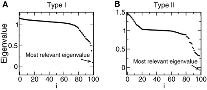
Figure 2. Examples of the eigenvalues of the matrix . The matrices are diagonalized and the eigenvalues are ordered from higher to lower. The most relevant eigenvalue is the one more separated from 1. (A) Type I network. (B) Type II network.

In the network, the role of stimulus s(t) is taken by the total current . As we will see below, in the balanced state the total input on any neuron has a Gaussian distribution and it could be directly used to perform covariance analysis. This technique has been developed for analyzing one neuron at a time. The main disadvantage is that in order to have enough statistics, at least several thousands spikes are needed, which implies very long recordings. On the other hand if we have a large network, it would be possible to collect a large number of spikes in a short time by recording simultaneously a large number of neurons. This is what we do in the present work. Of course, mixing spikes from an arbitrary set of neurons is not theoretically justified because their inputs can have different statistical properties. However we can make use of the fact that in the balanced state the statistical properties of the inputs are completely controlled by the mean firing rate of the neurons. This can be seen from the analysis in (Lerchner et al., 2006). Using the scaling of the synaptic efficacies and the central limit theorem it is found that the inputs have fluctuations with static and dynamic components. The total input can be written as

where U_k is a constant, x_i is a Gaussian random variable with zero mean and variance 1 that does not depend on time and is uncorrelated across neurons and y_i(t) is a Gaussian random variable with zero mean. The constant U_k, the variance of the static noise (B_k) and the autocorrelation function of the dynamic component can be evaluated self-consistently (see Lerchner et al., 2006 for the details). The autocorrelation functions are the same for all the neurons in a given population. This means that all the neurons in one population that have the same value of x_i will have the same input statistics and they will have the same average firing rate. If M identical neurons receive a set of inputs during a time T with the same statistical properties, then the STAs and the matrices C_prior and C_spikes evaluated by combining the vectors from all these neurons will give the same result as for one neuron during a time MT. In other words, it is approximately the same to do a very long simulation recording only one neuron than to do a shorter simulation recording a set of neurons that have very similar firing rates.

2.4 Characterization of the Dynamical State

The dynamical state of large network of conductance based neurons will differ from the theoretical predictions for the balanced state for several reasons. On the one hand we are limited to a finite number of neurons (N_k) and finite values of connectivity (K). On the other hand conductance based neurons have an internal dynamics with several time constants, in contrast with the binary neurons where the state is determined instantly by the strength of the input. And finally, synaptic interactions are also characterized by their own time constants. Therefore we need to characterize the dynamical state to see if we are under (or near) the conditions given by the balanced state.

The criteria we analyze are the following:

• The dependence of the average firing rate of each population on the external input. The prediction of the balanced state theory is that independently of the neuron dynamics, the average firing rate should be a linear function of the input.

• The scaling of different components of the total synaptic input for individual neurons on the connectivity. The prediction of the theory is that the total excitatory and inhibitory inputs should increase as the square root of the connectivity.

• The statistics of the synaptic input for individual neurons. The distribution should be Gaussian.

The autocorrelation function of the total synaptic input to neuron i in population k is defined by

The autocorrelation time (τ_AC,ik) is evaluated by

Let us note that if AC_ik(τ) has a purely exponential decay: AC_ik(τ)∝ exp(−τ/τ₀) and T ≫ τ₀ then we recover τ_AC,ik = τ₀.

2.5 Individual Neurons with Gaussian Input Noise

We compare the statistical results obtained with neurons from the different networks with individual neurons with Gaussian input noise. We simulate one cell with an input current given by

where <I> is the DC term, σ is the variance, and ξ is a Gaussian noise. The noise ξ(t) is such that (<ξ(t)> = 0 and . This input current has three parameters to be set: <I>, σ and τ_AC. These parameters can be determined from the statistics of the input that one neuron (or a group of neurons) receives in the network. Let us note that we are assuming here a purely exponential dependency for the autocorrelation. The discrepancies between the results for the simulation in the network with the individual neurons with Gaussian input noise will therefore reflect additional correlations, such as oscillatory components in the input. The comparison can be done in two different ways. In the first we compare one neuron in the network with one neuron with Gaussian input noise. In this case the duration of the simulation is the same in both cases. In the second we compare a group of neurons in the network (that have similar firing rates) with one neuron with Gaussian input noise. In this second case, as we combine all the spikes from the group to evaluate the STA and the matrix , the simulation of one neuron with Gaussian noise must be longer to obtain similar statistics as in the network simulation.

2.6 Simulation Methodology

In all the results the network has N_E = 16000 excitatory neurons and N_I = 4000 inhibitory neurons. The simulations were performed using a fourth-order Runge–Kutta algorithm (Press et al., 1992) with a time step of 0.01 ms. We checked that taking smaller time steps does not affect the results. The initial conditions are chosen randomly and there is a transient of 50 ms before recording the values of the membrane potential and the synaptic currents. These values are written every 0.5 ms. The total simulation time for each set of parameters was 50 s for Figures 3–5 and 300 s for Figures 6–12. We detect every time there is a spike when the membrane potential crosses the value 0 mV with positive slope. At that point we record the values of the excitatory and inhibitory currents during the previous 50 ms. These vectors (each one with N = 100 components) are used to evaluate the STA and the matrix C_spikes. We use only the spikes that are separated from the previous one in the same neuron by at least 50 ms. We also record the same vectors of excitatory and inhibitory currents every 500 ms without concern if there is a spike at the end or not. These vectors are used to evaluate the matrix C_prior.

FIGURE 3

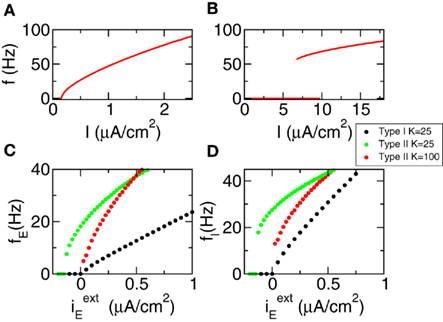
Figure 3. The f–I curves of the populations approach a linear behavior for large connectivity. (A) f–I curve of Type I neurons. (B) f–I curve of Type II neurons. (C) Mean activity of the excitatory population (D) Mean activity of the inhibitory population. Black dots: Type I network with K = 25. Green dots: Type II network with K = 25. Red dots: Type II network with K = 100.

3 Results

3.1 Characterization of the Dynamical State

We first show the results regarding the characterization of the dynamical state. We analyze Type I and Type II networks. In Figures 3A,B we show the f–I curve for both neurons. We can see that they are very different. The first one is continuous while the second is discontinuous and with a bistable region. In Figures 3C,D we show the mean network activity as a function of the external input (keeping ), see Eq. 4. We can see that for Type I neurons even a connectivity K = 25 is enough to transform the f–I curve of the individual neuron in almost a linear one at the population level. We can also see that, as predicted by the theory of the balanced state, the threshold is now at zero current. The behavior for Type II neurons is quantitatively different. Connectivity K = 25 is not enough to suppress the discontinuity of the f–I curve at the population level. But taking K = 100 strongly reduces the minimal average firing rate and makes the f–I population curves more similar to the theoretical prediction.

We can also analyze the dynamical state from the point of view of the total excitatory and inhibitory inputs on an individual neuron. For Type I networks we performed simulations with connectivity K = 25, 100, and 400, and for each case we choose a neuron with an average firing rate of about 30 Hz. Traces are shown in Figure 4A. In Figure 4B we can see the total excitatory and inhibitory inputs. As connectivity grows the individual components increase as predicted by the theory, with the square root of K. On the other hand the net result is almost the same, showing the cancelation between the two components. For Type II neurons the behavior is more complex. As connectivity grows the network tends to develop synchronized oscillations that manifest themselves in periodic fluctuations of the total currents on any given neuron. The value of the connectivity where this phenomenon arises depends on the network parameters. For instance for g_II = −30 μA ms/cm² this happens between K = 25 and K = 100 (Figures 4C,D). Taking a more negative value of g_II allows us to increase the connectivity. For instance for g_II = −45 μA ms/cm² the instability occurs between K = 100 and K = 400 (Figures 4E,F). The possibility of losing the balanced state because of oscillatory instability has been analyzed in (van Vreeswijk and Sompolinsky, 1998), where it is found that the instability depends on the couplings and the time constants of the populations. Here we find that balanced states in Type I networks are much more robust with respect to this instability than Type II networks. This is consistent with the results, shown for instance in (Ermentrout, 1996; Galan et al., 2007), that Type II neurons (resonators) synchronize more reliably and more robustly than Type I neurons (integrators).

FIGURE 4

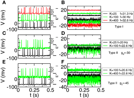
Figure 4. The positive and negative inputs to one neuron tend to cancel even as they grow stronger with larger connectivity. For Type II networks synchronized oscillations are found if connectivity is above some threshold. Left panels: traces of one neuron. Different curves have been shifted by 100 mV. Right panels: total excitatory (curves above 0) and inhibitory (curves below 0) currents (in μA/cm²). (A,B) Type I network with K = 25 (black), K = 100 (green), and K = 400 (red) . (C,D) Type II network with g_II = −30 μA ms/cm². K = 25 (black) and K = 100 (green). (E,F) Type II network with g_II = −45 μA ms/cm². K = 100 (black) and K = 400 (green). . Other parameters in Table A1 of Section 3 in Appendix.

Another of the predictions of the theory is that the total input to a given neuron should have a Gaussian distribution. To check this we evaluate the histogram of these inputs for neurons in the excitatory population and in the inhibitory population. The results are shown in Figure 5 for the mixed network. Similar results are obtained for Type I and Type II networks in the regime where there are no oscillations. Black curves show the results for two WB neurons (that are 95% of the E population and 5% of the I population) and red curves the results for two HH neurons (that are 5% of the E population and 95% of the I population). Figures 5A,B show that the distribution is approximately Gaussian with mean values and variances given in the inset of the figure. Figures 5C,D panels show the autocorrelation functions for the same neurons and the autocorrelation time evaluated according to Eq. 16. We can see that the autocorrelation is dominated by a fast decay term (that gives rise to an autocorrelation time between 1 and 2 ms) but there is a very small additional oscillatory component with a period of about 20 ms.

FIGURE 5

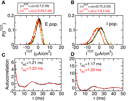
Figure 5. The inputs to one neuron have a statistics that is approximately Gaussian with a short autocorrelation time. Mixed network. (A,B) Histograms of total input on one neuron. Black: WB neuron. Red: HH neuron. Left panels: Excitatory population. Right panels: Inhibitory population. Insets show the mean value and variance of each curve in μA/cm². In yellow: Gaussian functions with the corresponding values of <I> and σ. (C,D) autocorrelation function of the total input for the same cases as in the upper panels. Parameters in Table A2 of Section 3 in Appendix.

A crucial prediction of the balanced state theory is that identical neurons with the same firing rate have total inputs with the same statistical properties, i.e., the same mean value and variance. Moreover, comparing different firing rates in a given population we should see that only the mean value changes but not the variance. To test these facts we divided each population according to the average firing rate of the neurons. The firing rate intervals were divided in windows with a fixed width. For each neuron we evaluated the mean value and variance of the total input current and then averaged those results over all the neurons with an average firing rate inside a given window. We show the results in Figure 6 (Figure 6A for Type I networks and Figure 6B for Type II networks). In each case the error bars represent the variance of the result over the corresponding subpopulation. We can see that the predictions of the balanced state theory are verified. On the one hand neurons inside each subpopulation have a well defined value of average total current and variance, with a small relative error. On the other hand, changing the firing rate affects strongly the mean value of the current but not the variance. It is interesting to notice that this condition is satisfied more precisely for Type II networks than for Type I networks. The same behavior is observed for the autocorrelation time. We can see that it is almost independent on the firing rate and also that all the neurons in a given window have the same autocorrelation time, giving rise to very small error bars. In fact, for Type II neurons the error bars are about 1% of the autocorrelation time. These results prove that neurons in a firing rate window have the same statistical properties and therefore their inputs can be combined to perform covariance analysis as proposed in the previous section. We must remark that this result is valid only if all the neurons in a given population are identical (i.e., they have the same dynamical behavior). In the last section we will discuss how this assumption limits the pooling of spike trains for the covariance analysis.

FIGURE 6

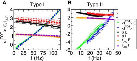
Figure 6. The average firing rate of the neurons is controlled by the average value of the total input, while the variance and the autocorrelation time are almost constant. Each point represents an average over a subpopulation of neurons with firing rate in a given window. The widths of the windows are: 3.1 Hz (Type I, E pop.), 4.2 Hz (Type I, I pop.), 0.63 Hz (Type II, E pop.), 0.65 Hz (Type II, I pop.). (A) Type I network. (B) Type II network. Green: mean value of the total current (E pop.). Blue: mean value of the total current (I pop.). Black: variance of the total current (E pop.). Red: variance of the total current (I pop.). Orange: average autocorrelation time (E pop.). Violet: average autocorrelation time (I pop.). Mean values and variances in μA/cm². Autocorrelation time in ms. As the average firing rate of the E pop. is lower than the firing rate of the I pop. the green, black and orange dots appear at lower firing rates than the blue, red, and violet points.

We finally show in Figure 7 the autocorrelation functions of neurons in Type I and Type II networks. For the purpose of comparison with the results of the covariance analysis we show the autocorrelation functions averaged over subpopulations of neurons with similar firing rate and not for individual neurons. The results obtained from for individual neurons are qualitatively similar but slightly noisier. The parameters are in Table A1 of Section 3 in Appendix. Let us note that keeping the same values of coupling parameters, autocorrelations in Type II networks show slightly stronger oscillations than in Type I networks. This is compatible with the results shown in Figure 4.

FIGURE 7

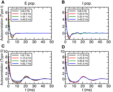
Figure 7. Autocorrelation functions of the total inputs averaged over a subpopulation of neurons with similar firing rates. (A,B) Type I networks. (C,D) Type II networks. Left panels: E population. Right panels: I population. The firing rate windows are centered around the values shown in the inset and the widths are: 3.1 Hz (Type I, E pop.), 4.2 Hz (Type I, I pop.), 0.63 Hz (Type II, E pop.), 0.65 Hz (Type II, I pop.).

3.2 Spike Triggered Average in the Mixed Network

We now analyze the inputs to individual neurons in the mixed network. As we have seen in Figure 5 the total input has a distribution that is approximately Gaussian and a short autocorrelation time. We use the inputs that precede the spikes to evaluate the STA using Eq. 11. In Figure 8 we show the results for four different neurons. In Figure 8A we show two neurons in the excitatory population. The black curve corresponds to a WB neuron (such neurons are 95% of this population) and the red one is an HH neuron (5% of the population). The error bars represent the statistical error of the STA at each point. In Figure 8B we show the two neurons in the inhibitory population, using the same convention. We can see that in both cases the STA of the HH neurons display a significant negative region, in contrast to the WB neurons. In order to test quantitatively this feature we have chosen the following criterion: we classify a neuron as Type II if the minimum value of the STA is below the average of the STA over the interval [−50:−25] ms by an amount that is larger than five times the average of the variance over the same interval. If this criterion is not satisfied we say the neuron is Type I. Applying this criterion to the neurons of Figure 8 gives the right classification. We have analyzed systematically all the neurons in the network and we have found an error rate of 7.4%, i.e., 92.6% of the neurons can be correctly classified using this simple criterion.

FIGURE 8

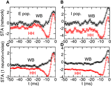
Figure 8. Spike triggered averages in the mixed case allow to determine the identity of the neuron. (A,B) Spikes triggered average of a two neurons. Black: WB neuron. Red: HH neuron. Left panel: neurons in the excitatory population. Right panel: neurons in the inhibitory population. (C,D) Spike triggered averages of individual neurons with purely Gaussian input (see Eq. 17). The parameters of the noise (mean value, variance, and autocorrelation time) are determined by the statistics of the neurons in the upper panels.

We compared the STA obtained from the network simulation with the one obtained from individual neurons that receive as input Gaussian noise with a mean value, variance, and autocorrelation time determined from the input in the network (see Eq. 17). The results are shown in panels C and D. We can see that these “isolated neuron” STAs are qualitatively similar to the ones seen in the network. This shows that the non-Gaussian effects and the non-exponential part of the autocorrelation functions are small enough not to affect significantly the results.

3.3 Spike Triggered Average and Covariance Analysis in Type I Networks

We now analyze the dependence of the STA and the relevant features identified by the covariance analysis on firing rate. In Figures 9A,B we show the STA averaged over a subpopulation of neurons whose frequencies are in a window around the firing rate shown in the inset (width of the windows in the caption). We show four cases, with firing rates going from 6.2 to 46.5 Hz (excitatory population, left panel) and 8.3 to 46 Hz (inhibitory population, right panel). We can see that the STA shows only a very weak dependence on the firing rate. This seems to be in contradiction with the results found in (Mato and Samengo, 2008), where it is shown that as firing rate grows the STA becomes sharper. The reason for the discrepancy is that in that case the firing rate is controlled by changing the variance of the noise, while here the most important factor is the change in the mean value of the input current. To check this interpretation we have performed simulations of one neuron with Gaussian noise. The parameters of the noise are determined by averaging the mean value, variance, and autocorrelation time of the total input to each one of the neurons inside one group. The results are shown in Figures 9C,D. We can see again that the STA does not depend substantially on the firing rate when the parameters of the noise are the ones given in Figure 6.

FIGURE 9

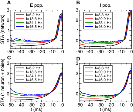
Figure 9. Spike triggered averages in Type I networks do not depend on firing rate and can be predicted from simulations of isolated neurons with noise. (A,B) STA averaged over a subpopulation of neurons with similar firing rate. Left: E population, right I population. Width of the firing rate windows: 3.1 and 4.2 Hz respectively. (C,D) STA of a single neuron with Gaussian noise. Parameters of the noise obtained from averaging the parameters (<I>, σ, τ_AC) of each subpopulation. For clarity error bars are not shown.

Similar results are obtained for the most relevant eigenvectors (see Section 3) in the covariance analysis. In this case we do not perform the analysis for individual neurons. The reason is that covariance analysis requires very good statistics in order separate the relevant eigenvalues from the background. Typically tens or hundreds thousand spikes are required (Agüera y Arcas et al., 2003), and performing extremely long simulations of large networks is impractical. Instead, because of the statistical properties of the balanced state mentioned in Section 3 and verified by the results in Figure 6, we can improve the statistics by averaging over a subpopulation of neurons with similar firing rates. In Figures 10A,B we show the most relevant eigenvector for the different firing rates. In this case the covariance and prior matrices (Eqs 10 and 12) are evaluated using all the vectors in the neurons that belong to the corresponding firing rate window. As we have mentioned in the previous section, this is justified by the fact that the inputs have essentially the same statistical properties if the firing rate is the same. In the lower panels we show the most relevant eigenvector for the simulation of one neuron with Gaussian noise, as in the previous figure.

FIGURE 10

Figure 10. Relevant eigenvectors in Type I networks do not depend on firing rate and can be predicted from simulations of isolated neurons with noise. (A,B) Most relevant eigenvector of a subpopulation of neurons with similar firing rate. Left: E population, right I population. Width of the firing rate windows: 3.1 and 4.2 Hz respectively. (C,D) Most relevant eigenvector of a single neuron with Gaussian noise. Parameters of the noise obtained from averaging the parameters (<I>, σ, τ_AC) of each subpopulation.

3.4 Spike Triggered Average and Covariance Analysis in Type II Networks

We now show the results for Type II networks. As we have seen in Section 1 Type II networks have a strong tendency to develop synchronized oscillations. These oscillations appear both in the STA and in the relevant eigenvalues. As in the previous case we compare the STA and the most relevant eigenvector from a group of neurons with a similar firing rate to the same functions obtained from a neuron that receives Gaussian noise.

In Figure 11 we see the results for the STA. We observe that for all the firing rates the STA displays a significant trough characteristic of Type II neurons (Mato and Samengo, 2008). However now there is a significant difference between the network simulations (Figures 11A,B) and the one neuron simulations (Figures 11C,D). The STA from the network simulation displays a more oscillatory shape, with a positive component in the range [−30:−20] ms. This component does not appear in the one neuron simulation and therefore is a manifestation of the oscillatory input.

FIGURE 11

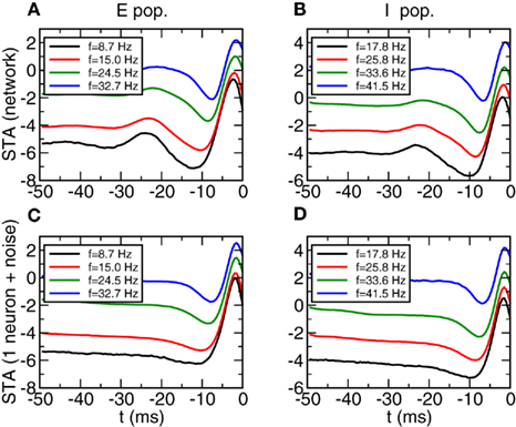
Figure 11. Spike triggered averages in Type II networks depend only weakly on firing rate. (A,B) STA averaged over a subpopulation of neurons with similar firing rate. Left: E population, right I population. Width of the firing rate windows: 0.63 and 0.65 Hz respectively. (C,D) STA of a single neuron with Gaussian noise. Parameters of the noise obtained from averaging the parameters (<I>, σ, τ_AC) of each subpopulation. For clarity error bars are not shown.

Similar results are obtained for the most relevant eigenvector. See Figure 12. The network simulation shows a more oscillatory behavior in the network evolution than in the one neuron simulation. But in any case the curves are essentially the same in the range [−15:0] ms. This shows, that independently of the synchronized oscillations of the input it is possible to identify without ambiguity the type of intrinsic neuron dynamics. Let us note that the discrepancies between the results from the network and the results from the isolated neuron can be understood looking at the autocorrelation functions from Figures 7C,D. The excess autocorrelation at about 20 ms translates into the additional STA at −20 ms, and also affects the relevant eigenvector. In contrast, Type I autocorrelations are much flatter and there is no significant discrepancy between relevant features in the network and in the isolated neuron.

FIGURE 12

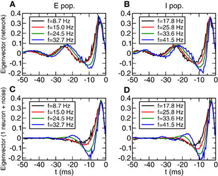
Figure 12. Spike triggered averages in Type II networks depend only weakly on firing rate. (A,B) Most relevant eigenvector of a subpopulation of neurons with similar firing rate. Left: E population, right I population. Width of the firing rate windows: 0.63 and 0.65 Hz respectively. (C,D) Most relevant eigenvector of a single neuron with Gaussian noise. Parameters of the noise obtained from averaging the parameters (<I>, σ, τ_AC) of each subpopulation.

4 Discussion

We have analyzed the dynamical behavior of large networks of conductance based neurons. The network parameters (connectivity, synaptic strength) are chosen in such a way that the system is approximately in a balanced state. This approximation is clearly better for Type I neurons (such as WB) than for Type II neurons (such as HH). On the one hand Type II networks require a higher connectivity to suppress the discontinuity of the f–I curve found in the individual neuron and also these networks have a stronger tendency to develop synchronized oscillations. But in both cases we can easily find situations where the total neuronal input has a statistical distribution that is approximately Gaussian and with an autocorrelation function that is dominated by a short exponential decay. We have also studied additional aspects of the dynamical behavior such as the cross-correlations of the inputs to different neurons. We have found that these cross-correlations are extremely small, with normalized cross-correlations coefficients (cross-correlation functions divided by the product of the variances) always less than 3% (which is in agreement with the results of Hertz, 2010). We have not shown these data because they are not directly relevant for the identification of single neuron properties, but they lead to the same conclusion as before, that we are approximately in a balanced state.

Even if we are not in the perfectly ideal conditions of the theory of the balanced state (van Vreeswijk and Sompolinsky, 1998) we can use the noisy input to evaluate STAs and perform covariance analysis (Agüera y Arcas and Fairhall, 2003; Bialek and De Ruyter von Steveninck, 2003; Paninski, 2003). We have found that under reasonably realistic conditions the results of this analysis closely resemble the result one would obtain from single neuron simulations with external Gaussian noise. Let us remark that this is the standard way of performing covariance analysis and feature extraction. For the cases we have analyzed this is enough to discriminate the different neuronal types. As far as we know this is the first method that allows the identification of neuron properties inside a network without any external stimulation, besides the constant currents . We have tested that reverse correlation methods can be used even in “mixed” networks, where a small fraction of neurons of one population differs from the dominant type. In these cases, evaluating the STA of individual neurons allows to make a prediction with an error rate lower than 10%. In principle, improving the statistics would allow to extract even more information about the neuronal dynamics. Using our technique we have found that a few hundred seconds of simulations are required to discriminate a second eigenvector, although we have not performed a systematic analysis of its properties.

As a very good statistics is required for the evaluation of the eigenvectors of the covariance matrix, we have not performed this analysis for individual neurons but for subpopulations of neurons with similar firing rates. This can be justified theoretically from the statistical properties of the balanced state. This pooling of spike trains from different neurons can be performed only if the neurons are identical. If they are not we cannot infer from the firing rate itself that the statistics of the input currents are the same. However the method could be used even if homogeneity of neurons in each population cannot be assumed. This could be done by performing preliminary measurements of the STA and the statistics of the input. Combining data from several neurons in which these quantities are very similar would still be valid, assuming that similar STAs reflect similar intrinsic dynamics. The purpose of implementing this procedure would be to extract more detailed information than the one given by the STA by itself. As it is shown, for instance, in (Mato and Samengo, 2008) the study of additional eigenvectors in Type II neurons gives information of the different intrinsic frequencies in the model.

Besides the assumption of homogeneity, another possible concern regarding the validity of the findings is that we are using current based synapses instead of the more realistic conductance based synapses. These synapses have been shown to be problematic in balanced states because when they are very strong they can generate a very small effective time scale that, interacting with a finite autocorrelation time in the input current, originates bursting firing patterns with long autocorrelation times. This problem is really severe for linear integrate-and-fire neurons, as shown in (vanVreeswijk:2003]). However, for conductance based neurons it is expected that the problem is not so severe because the absolute or relative refractory periods of the intrinsic neuron dynamics will control the bursts. In (Hertz, 2010) conductance based networks with conductance based synapses are simulated with network sizes and connectivities similar to ours, and no bursting behavior is found, suggesting that the balanced state has not been substantially altered by the conductance based synapses. We have performed some simulations with conductance based synapses and found a similar qualitative behavior as for current based synapses. Input currents have a distribution that is approximately Gaussian and STAs are very similar to the results shown here. Therefore they can be used to discriminate between the different neuronal types. We also checked that the autocorrelation time of the input is of order of 1 ms (let us note that Hertz, 2010 obtains a few milliseconds for a different model).

Summarizing, we have shown that an approximate balanced state allows the use reverse of correlation methods to infer intrinsic neuronal properties. This state can be achieved in realistic conditions for a wide variety of networks. The method could be applied to extract information of the neuron properties without external perturbations.

Conflict of Interest Statement

The authors declare that the research was conducted in the absence of any commercial or financial relationships that could be construed as a potential conflict of interest.

Acknowledgments

We thank Guillermo Abramson and Inés Samengo for a careful reading of the manuscript. This work has been supported by the Comisión Nacional de Investigaciones Científicas y Técnicas (PIP 112 200901 00738) and the Universidad Nacional de Cuyo (research project 06/C308).

References

Agüera y Arcas, B., and Fairhall, A. L. (2003). What causes a neuron to spike? Neural Comput. 15, 1789–1807.

Pubmed Abstract | Pubmed Full Text | CrossRef Full Text

Agüera y Arcas, B., Fairhall, A. L., and Bialek, W. (2003). Computation in single neuron: Hodgin and Huxley revisited. Neural Comput. 15, 1715–1749.

Pubmed Abstract | Pubmed Full Text | CrossRef Full Text

Baroni, F., and Varona, P. (2007). Subthreshold oscillations and neuronal input-output relationships. Neurocomputing 70, 1611–1614.

CrossRef Full Text

Bialek, W., and De Ruyter von Steveninck, R. R. (2003). Features and dimensions: motion estimation in fly vision. arXiv:q-bio/0505003.

Brown, E., Moehlis, J., and Holmes, P. (2004). On the phase reduction and response dynamics of neural oscillator populations. Neural Comput. 16, 673–715.

Pubmed Abstract | Pubmed Full Text | CrossRef Full Text

Ermentrout, B. (1996). Type I membranes, phase resetting curves, and synchrony. Neural Comput. 8, 979–1001.

Pubmed Abstract | Pubmed Full Text | CrossRef Full Text

Galan, R. F., Ermentrout, G. B., and Urban, N. N. (2007). Reliability and stochastic synchronization in type I vs. type II neural oscillators. Neurocomputing 70, 2102–2106.

CrossRef Full Text

Hertz, J. (2010). Cross-correlations in high-conductance states of a model cortical network. Neural Comput. 22, 427–447.

Pubmed Abstract | Pubmed Full Text | CrossRef Full Text

Hodgkin, A. L. (1948). The local electric charges associated with repetitive action in non-medullated axons. J. Physiol. (Lond.) 107, 165–181.

Pubmed Abstract | Pubmed Full Text

Hodgkin, A. L., and Huxley, A. F. (1952). A quantitative description of membrane current and application to conductance in excitation nerve. J. Physiol. (Lond.) 117, 500–544.

Pubmed Abstract | Pubmed Full Text

Holt, G. R., Softky, W. R., Koch, C., and Douglas, R. J. (1996). Comparison of discharge variability in vitro and in vivo in cat visual cortex neurons. J. Neurophysiol. 75, 1806–1814.

Pubmed Abstract | Pubmed Full Text

Hong, S., Agüera y Arcas, B., and Fairhall, A. (2007). Single neuron computation: from dynamical system to feature detector. Neural Comput. 19, 3133–3172.

Pubmed Abstract | Pubmed Full Text | CrossRef Full Text

Izhikevich, E. (2001). Resonate and fire neurons. Neural Netw. 14, 833–894.

CrossRef Full Text

Izhikevich, E. (2007). Dynamical Systems in Neuroscience. The Geometry of Excitability and Bursting. Cambridge, MA: The MIT Press.

Koch, C. (1999). Biophysics of Computation: Information Processing in Single Neurons. New York: Oxford University Press.

Lerchner, A., Ursta, C., Hertz, J., Ahmadi, M., Ruffiot, P., and Enemark, S. (2006). Response variability in balanced cortical networks. Neural Comput. 18, 634–659.

Pubmed Abstract | Pubmed Full Text | CrossRef Full Text

Maravall, M., Petersen, R. S., Fairhall, A. L., Arabzadeh, E., and Diamond, M. E. (2007). Shifts in coding properties and maintenance of information transmission during adaptation in barrel cortex. PLoS Biol. 5, e19.

Pubmed Abstract | Pubmed Full Text | CrossRef Full Text

Mato, G., and Samengo, I. (2008). Type I and type II neuron models are selectively driven by differential stimulus features. Neural Comput. 20, 2418–2440.

Pubmed Abstract | Pubmed Full Text | CrossRef Full Text

Muresan, R. C., and Savin, C. (2007). Resonance or integration? Self-sustained dynamics and excitability of neural microcircuits. J. Neurophysiol. 97, 1911–1930.

Pubmed Abstract | Pubmed Full Text | CrossRef Full Text

Paninski, L. (2003). Convergence properties of some spike-triggered analysis techniques. Network 14, 437–464.

Pubmed Abstract | Pubmed Full Text | CrossRef Full Text

Press, W. H., Teukolsky, S. A., Vetterling, W. Y., and Flannery, B. P. (1992). Numerical Recipes in Fortran 77. Cambridge, UK: Cambridge University Press.

Reyes, A., Lujan, R., Rozov, A., Burnashev, N., Somogyi, P., and Sakmann, B. (1998). Target-cell-specific facilitation and depression in neocortical circuits. Nat. Neurosci. 1, 279–285.

Pubmed Abstract | Pubmed Full Text | CrossRef Full Text

Rozov, A., Burnashev, N., Sakmann, B., and Neher, E. (2001). Transmitter release modulation by intracellular Ca2+ buffers in facilitating and depressing nerve terminals of pyramidal cells in layer 2/3 of the rat neocortex indicates a target cell-specific difference in presynaptic calcium dynamics. J. Physiol. (Lond.) 531, 807–826.

Pubmed Abstract | Pubmed Full Text | CrossRef Full Text

Rust, N. C., Schwartz, O., Movshon, J. A., and Simoncelli, E. P. (2005). Spatiotemporal elements of macaque V1 receptive fields. Neuron 46, 945–956.

Pubmed Abstract | Pubmed Full Text | CrossRef Full Text

Schwartz, O., Pillow, J. W., Rust, N. C., and Simoncelli, E. P. (2006). Spike-triggered neural characterization. J. Vis. 6, 484–507.

Pubmed Abstract | Pubmed Full Text | CrossRef Full Text

Softky, W. R., and Koch, C. (1993). The highly irregular firing of cortical cells is inconsistent with temporal integration of random EPSPs. J. Neurosci. 13, 334–350.

Pubmed Abstract | Pubmed Full Text

Tateno, T., Harsch, A., and Robinson, H. P. C. (2004). Threshold firing frequency current relationships of neurons in rat somatosensory cortex: type 1 and type 2 dynamics. J. Neurophysiol. 92, 2283–2294.

Pubmed Abstract | Pubmed Full Text | CrossRef Full Text

Tateno, T., and Robinson, H. P. C. (2006). Rate coding and spike-time variability in cortical neurons with two types of threshold dynamics. J. Neurophysiol. 95, 2650–2663.

Pubmed Abstract | Pubmed Full Text | CrossRef Full Text

van Vreeswijk, C., and Sompolinsky, H. (1996). Chaos in neuronal networks with balanced excitatory and inhibitory activity. Science 274, 1724–1726.

Pubmed Abstract | Pubmed Full Text | CrossRef Full Text

van Vreeswijk, C., and Sompolinsky, H. (1998). Chaotic balanced state in a model of cortical circuits. Neural Comput. 10, 1321–1371.

Pubmed Abstract | Pubmed Full Text | CrossRef Full Text

van Vreeswijk, C., and Sompolinsky, H. (2003). “Irregular activity in large networks of neurons,” in Methods and Models in Neurophysics, Lecture Notes of the XXX Les Houches Summer School, eds C. Chow, B. Gutkin, D. Hansel, C. Meunier, and J. Dalibard (London: Elsevier Science and Technology), 341–402.

Wang, X.-J., and Buzsáki, G. (1996). Gamma oscillation by synaptic inhibition in a hippocampal interneuronal network model. J. Neurosci. 16, 6402–6413.

Pubmed Abstract | Pubmed Full Text

Appendix

Wang–Buzsáki (WB) Model

The dynamical equations for the conductance based Type I neuron model used in this work were introduced by (Wang and Buzsáki, 1996). They are

The parameters g_Na, g_K, and g_l are the maximum conductances per surface unit for the sodium, potassium, and leak currents respectively and V_Na, V_K, and V_l are the corresponding reversal potentials. The capacitance per surface unit is denoted by C. The external stimulus on the neuron is represented by an external current I. The functions m_∞(V), h_∞(V), and n_∞(V) are defined as x_∞(V) = a_x(V)/[a_x(V) + b_x(V)], where x = m, n, or h. In turn, the characteristic times (in milliseconds) τ_n and τ_h are given by τ_x = 1/[a_x(V) + b_x(V)], and

The other parameters of the sodium current are: g_Na = 35 mS/cm² and V_Na = 55 mV. The delayed rectifier current is described in a similar way as in the HH model with:

Other parameters of the model are: V_K = −90 mV, V_Na = 55 mV, V_ℓ = −65 mV, C = 1 μF/cm², g_ℓ = 0.1 mS/cm², g_Na = 35 mS/cm², g_K = 9 mS/cm², ɸ = 3.

Hodgkin–Huxley (HH) Model

The dynamical equations of the Hodgkin–Huxley model (Hodgkin, 1948; Hodgkin and Huxley, 1952) read

For the squid giant axon, the parameters at 6.3°C are: V_Na = 50 mV, V_K = −77 mV, V_l = −54.4 mV, g_Na = 120 mS/cm², g_K = 36 mS/cm², g_l = 0.3 mS/cm², and C = 1 μrmF/cm². The functions m_∞(V), h_∞(V), n_∞(V), τ_m(V), τ_n(V), and τ_h(V), are defined in terms of the functions a(V) and b(V) as in the WB model, but now

Network parameters

The network sizes are N_E = 16000, N_I = 4000. The synaptic time constants are given by: , , τ_I = 2 ms. The external inputs are: for Type I, for Type II, and for mixed networks.

The rest for the parameters for Type I, Type II, and mixed networks are given in Tables A1 and A2.

TABLE A1

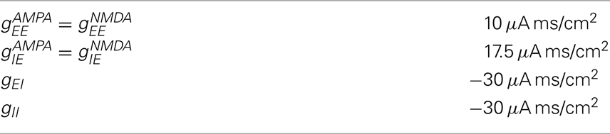
Table A1. Parameters for Type I and Type II networks.

TABLE A2

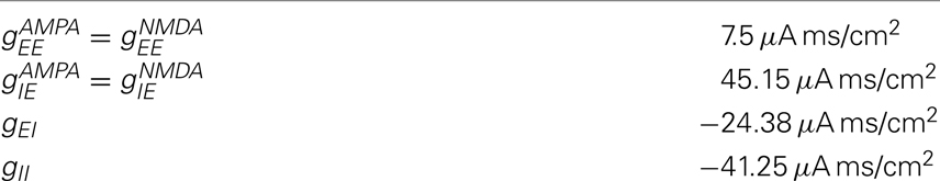
Table A2. Parameters for mixed networks.