Phase diagram of spiking neural networks

1. Introduction

A simulation of neural network consists of model neurons that interact via network parameters; The model is a set of differential equations that describes the behaviors of neurons and synapses, captured by years of electro physiological studies (Nicholls et al., 2012). A model can be as simple as Integrate-and-fire or as realistic as Hodgkin-Huxley (Sterratt et al., 2011). Realistic models generate reliable results, but they are computationally expensive. On the other hand, simple models consume less computer resources, at the cost of loosing details and biological plausibility; therefore, there is a delicate balance between computational feasibility and biological plausibility, Fortunately, there are many reviews and books that compare different models (Izhikevich, 2004; Herz et al., 2006; Sterratt et al., 2011) and neural simulators (Brette et al., 2007). They help us to find a suitable model of a single neuron, set its parameters, and get reliable results in a reasonable time.

No matter how much a neural model is detailed and efficient, A carelessly constructed networks of perfect neural models, is misleading. It only produces wrong biologically plausible results, in a reasonable time. Unfortunately, network parameters are a lot more ambiguous.

There are four essential parameters in a neural network simulation that I investigated in this work - the ratio of excitatory neurons to inhibitory neurons, the topology and sparseness of connections, inhibitory and excitatory synaptic weights. To make it more general and realistic, one may consider the values follow a distribution. This distribution function may change the behavior.

There are experimental works that reads network parameters from nature (Binzegger et al., 2004; Brown and Hestrin, 2009; Lefort et al., 2009; Ko et al., 2011; Perin et al., 2011; Feldmeyer, 2012). For example, Lefort et al studied the share of inhibitory neurons in each layer of C2 barrel column of mouse (Lefort et al., 2009). They reported that 100, 16, 10, 8, 17, 17, and 9 percent of layer 1, 2, 3, 4, 5A, 5B, and 6 are inhibitory neurons, and in total, 11 percents of the column is made of inhibitory neurons. They have also studied the synaptic connections of excitatory neurons, they reported neurons of each layers 2, 3, 4, 5A, 5B, and 6 is connected with the probability of 9.3, 18.7, 24.3, 19.1, 7.2, and 2.8 percents to the neurons of the same layer. Moreover, they have studied synaptic weights by measuring unitary Excitatory Post Synaptic Potential (uEPSP), the mean uEPSP for connections inside a layer are 0.64, 0.78, 0.95, 0.66, 0.71, and 0.53 mV for layer 2–6 but the maximum values are much larger, 3.88, 2.76, 7.79, 5.24, 7.16, and 3 mV for the same layers respectively.

The actual values in computer simulations usually are less diverse, In many computational studies, 20% of the neurons are inhibitory, the network topology is a random graph with sparseness of 2% and there are only a couple of fixed synaptic weights for inhibitory and excitatory neurons. Despite their simplicity, they observe many interesting phenomena like oscillations, synchrony, modulations (Song et al., 2000; Brette et al., 2007; Goodman and Brette, 2008; Buice and Cowan, 2009; Akam and Kullmann, 2010; Mejias and Longtin, 2012; Augustin et al., 2013) and even psychological disorders (Bakhtiari et al., 2012). There are also many works that show the results are not actually sensitive to the parameters (Prinz et al., 2004; Marder et al., 2007; Marder, 2011; Marder and Taylor, 2011; Gutierrez et al., 2013).

Why do this parameters appear in nature? What are their evolutionary advantages? How much is the result of a simulation robust in respect to the parameters? How does one decide about the network parameters in a simulation? Which other parameters might give the same results? These are few question that come to mind, while dealing with properties of neural networks, and they could be easily answered by looking at a phase diagram of neural networks, that shows the behavior of a network in respect to its parameters. Like the phase diagram of water, tells us about the properties of water in different pressures and temperatures. But such a phase diagram does not exist for spiking neural networks, yet. First, because of the large amount of computation needed and second, because of the ambiguity of the concept of phase or state in neural networks.

To answer these question, I could use sophisticated evolutionary algorithms, like the study of evolution of inteligence by McNally et al. (2012), however, I used a simple brute force search in the space of parameters, so I can also generate a phase diagram, similar to the work of Roy et al. (2013).

2. Method

I did a brute force search in the space of parameters, by simulating a population of 1000 neurons, let say a part of a single layer of cortex, that receives excitatory signals from previous layer of cortex or an external stimuli, and then sends excitatory signals to the next layer. There are lateral connections among all types of neurons (excitatory and inhibitory) in a single layer, but only excitatory neurons interconnects different layers. I stimulated this network and watched its response. This was repeated over a wide range of parameters. At the end I calculated fitness of each set of parameters and then investigated the overlap of the best parameters according to my simulation with the nature's choices (or computational neuroscientists' choices).

To do any sort of evolutionary analysis, first we need to agree on something to optimize –a fitness function, it can be the network capacity to learn and store information (Barbour et al., 2007), or it can be the speed and the quality of transmitted signals (Chklovskii et al., 2002). But here, to define the fitness function, I remind you of three obvious evolutionary facts:

1. High Dynamic Range is evolutionary favored, an animal that can see during days and nights, has a higher survival chance than an animal which can see only during days.

2. Small Just-Noticeable Difference is evolutionary favored, an animal which can discriminate more gray levels or colors, has a better chance to find its preys and foods.

3. Low Energy Consumption is also favored, an energy efficient animal, consumes less food and therefore has a better chance to survive (Niven and Laughlin, 2008).

Dynamic Range is the ratio of the largest possible value of stimuli to its smallest perceivable value. Just-Noticeable Difference is the smallest detectable difference between two sensory stimuli, which is often roughly proportional to the magnitude of the stimulus. The ratio of Just-Noticeable Difference to the magnitude of the stimulus is known as Weber constant (Dayan and Abbott, 2001).

Both Dynamic Range and Just-Noticeable are well presented in logarithmic scale, but instead of log₁₀ and dB, from now on, I will use log₂ and stop which are common in Optics and Photography (Figure 1).

FIGURE 1

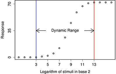
Figure 1. This figure demonstrates a typical tuning curve and its dynamic range. Two consecutive stimuli are different by a factor of 2, also known as one stop.

Here we are left with a neural network and three concepts to play with—Dynamic Range, Just-Noticeable Different and Energy Consumption. To keep it simple, I only measure Dynamic Range while there are upper bounds for the other two. I require Just-Noticeable Different to be smaller than one stop, thus, the calculated Dynamic Range is a lower bound for the real Dynamic Range, and I require the Energy Consumption to be zero in absence of stimulus, which puts an upper bound for the Energy Consumption. Moreover, energy consumption can be a determinant factor when all other conditions are equal, when there are two sets of parameters with about the same Dynamic Range, the one which consumed less energy will be favored, and here, the measure of energy consumption is the number generated spikes (Attwell and Laughlin, 2001).

I stimulated the network with a set of stimuli that were equally spaced in the logarithmic scale, separated by 1 stop (× 2) intervals, similar to Figure 1. I ran the simulation for a given time 1024 ms and then I calculated Dynamic Range over the range that Just-Noticeable Difference was smaller than 1 stop.

To be precise, I used a sequence of n stimuli plus the resting state (no stimulus), so the sequence includes n + 1 members s ϵ (s₀, s₁, s₂, …, s_n). Except s₀, the resting state, the difference between i-th and (i + 1)-th stimulus is one stop: s_{i + 1} = 2*s_i. Each stimulus s_i evokes a response r(s_i) ϵ R, where R = (r(s₀), r(s₁), r(s₂), …, r(s_n)). Now, the Dynamic Range is simply the number of elements in the largest subsequence of R′ ⊂ R that fulfills the expectations,

1. For any r(s_i), r(s_j) ϵ R′, we should have s_i < s_j ⇒ r(s_i) < r(s_j). It means that R′ is strictly monotonic and it satisfies the constrain on the Just-Noticeable difference.

2. For any s_i ϵ R′, the network must return to resting state in acceptable time. This satisfy the Energy Consumption constrains.

For example, if stimuli (0, 1, 2, 4, 8, 16) leads to the responses (0, 0, 2, 3, 4, 4) then the subsequence (0, 2, 3, 4) ⊂ R is the largest subsequence of R which meets all the conditions; Therefore, the dynamic range is 4. In this way the minumum dynamic range can be 1 and its maximum can reach the total number of stimuli.

In this study I assumed response r(s) as the maximum firing rate of population of excitatory neurons in response to the stimulus s. But the paradigm of this study is general and can be applied to any neural coding schemes.

I stimulated some of the neurons with an impulse, I forced s_i excitatory neurons to fire once at time t = 0, then I monitored the propagation of the impulse. Here the number of excited neurons represents the magnitude of the stimuli s_i. This is very similar to Optogenetics stimulation, in which, a laser pulse excites a specific population of neurons (Peron and Svoboda, 2011; Toettcher et al., 2011; Lim et al., 2012; Liu et al., 2012).

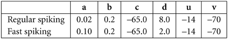
I used a simple compartment Izhikevic model (Izhikevich, 2003). It can imitate the behavior of Hodgkin-Huxley model, and its computational costs is comparable to the Integrate-and-fire model (Izhikevich, 2004). It is based on a system two-dimensional differential equations:

$\begin{array}{cc}\frac{dv}{dt}=0.04v^2+5v+140-u+I\hfill & (1)\end{array}$

$\begin{array}{cc}\frac{dw}{dt}=a(bv-u)& (2)\end{array}$

and the after spike equation of:

$\text{if }v>30\text{mV, then}\{\begin{array}{l}v\leftarrow c\hfill \\ u\leftarrow u+d\hfill \end{array}$

all units are in mV and ms. Here v is the membrane potential, I is the input current and u is a slow variable that imitate the effect of slow moving ions in the cell, like Calcium ions. With a proper values of parameters a, b, c, and d, it can model regular spiking neurons, fast spiking neurons and it includes adaptation. In our simulaton excitatory neurons are assumed to be regular spiking, inhibitory neurons are assumed to be fast spiking. The values of parameters and the initial values of u and v are set as follow:

My network has a random graph topology (Erds and Rényi, 1960). In a random graph, every two neurons are connected by probability p, called sparseness. This is one of the simplest topology for a network or graph.

I simulated networks of N = 1000 neurons with

$N_I\in (100,200,300,400,500)$

inhibitory neurons. The neurons were connected by a random graph topology, with the sparseness

$p\in (0.01,0.02,0.04,0.08,0.16).$

On the other hands, the synaptic weights are chosen randomly, but in a way to cover the region of interest in the w_e, w_i plane. In this way, it is always possible to add new points later to improve results. The new points could be just another pair of connection weights(w_e, w_i) on the same random netwrok, or they could be synaptic weights of a whole new realiziation.

I stimulated each network 10 times,

$s\in (0,1,2,4,8,16,32,64,128,256)$

so in each trial, s neurons fire at t = 0. Then I watched the network for 1024 ms. At the end, I calculated Dynamic Range of the network. I repeated the whole process for few realization of random networks and and then the median of all data in each hexagonal is calculated and displayed (Figure 2).

FIGURE 2

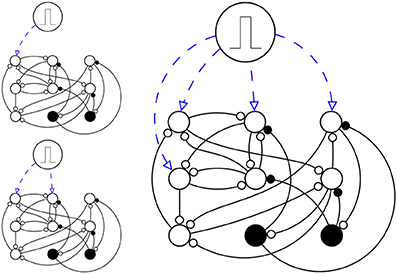
Figure 2. A simplified schema of simulation setup. Here there are just N = 9 neurons (N = 1000 in the actual simulation), in which N_e = 7 are excitatory neurons (circles) and N_i = 2 are inhibitory neurons (disks). The network is stimulated three times, each time s ϵ (1, 2, 4) neurons are stimulated (up left, down left and right respectively), with a pulse, in a way that they fire once at time t = 0 and then they are like any other neuron in the network.

The whole process needs a great amount of computational power. That is the reason I used NeMo (http://nemosim.sourceforge.net/), a neural simulator software that runs on GPU (Fidjeland et al., 2009; Fidjeland and Shanahan, 2010), but for the pilot study, I used Brian (http://briansimulator.org/) (Goodman and Brette, 2008). Both of them are open source and available on their websites.

3. Results

I wanted to present the results as a function of 4 other parameters, for that I needed to map a 4-D space to a 2-D space. Here I used the template in Figure 3, to present the dynamic ranges in Figure 4, oscillations in Figure 5, diuration of activities in Figure 6, maximum achived firing rate in each trial in Figure 7 and the time of achived maximum rate in Figure 8 First I made the plots of dynamic range in the space of synaptic weights – w_e and w_i. Then I put these plots next to each other according to sparseness of connections p and number of inhibitory neurons N_i.

FIGURE 3

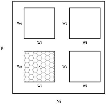
Figure 3. The layout of phase diagram, (Figure 4 and others), Here, p is the sparsness of connections, N_i is the number of inhibitory neurons, w_e is the weight of excitatory synapses (a positive number) and w_i is the weight of inhibitory synapses (a negative number). The plane of w_e and w_i is devided into hexagonal bins. The color of each hexagon is defined by the aggregated value of data points inside that hexagon. For aggregation, unless spesified, median value of points are used. If a hexagon is empty, then its color is white.

FIGURE 4

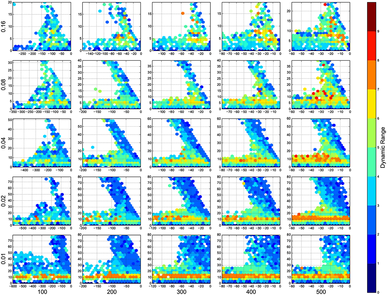
Figure 4. The phase diagram of dynamic ranges, dark red means high dynamic range (good), white means there was not any simulation data at that bin, all the data were unreliable, or the the network did not come back to its resting state before 100 ms of simulation. The information are arranged according to the template of Figure 3.

FIGURE 5

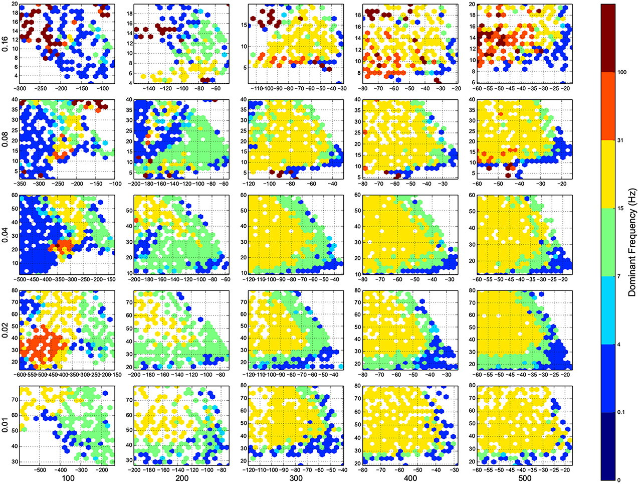
Figure 5. The phase diagram of oscillations, the dominant frequency of population rate of the network acording to FFT. Colors are associated to brain waves: δ (0.1-4 Hz), θ (4-7 Hz), α (7-15 Hz), β (15-31 Hz), and γ(31-100 Hz), and color of a bin shows the median of all trials in that bin. Here white means there was not any simulation data at that bin, all the data were unreliable (they fired at the maximum possible population firing rate), or the network did not show any activity after 100 ms of simulation. The information are arranged according to the template of Figure 3.

FIGURE 6

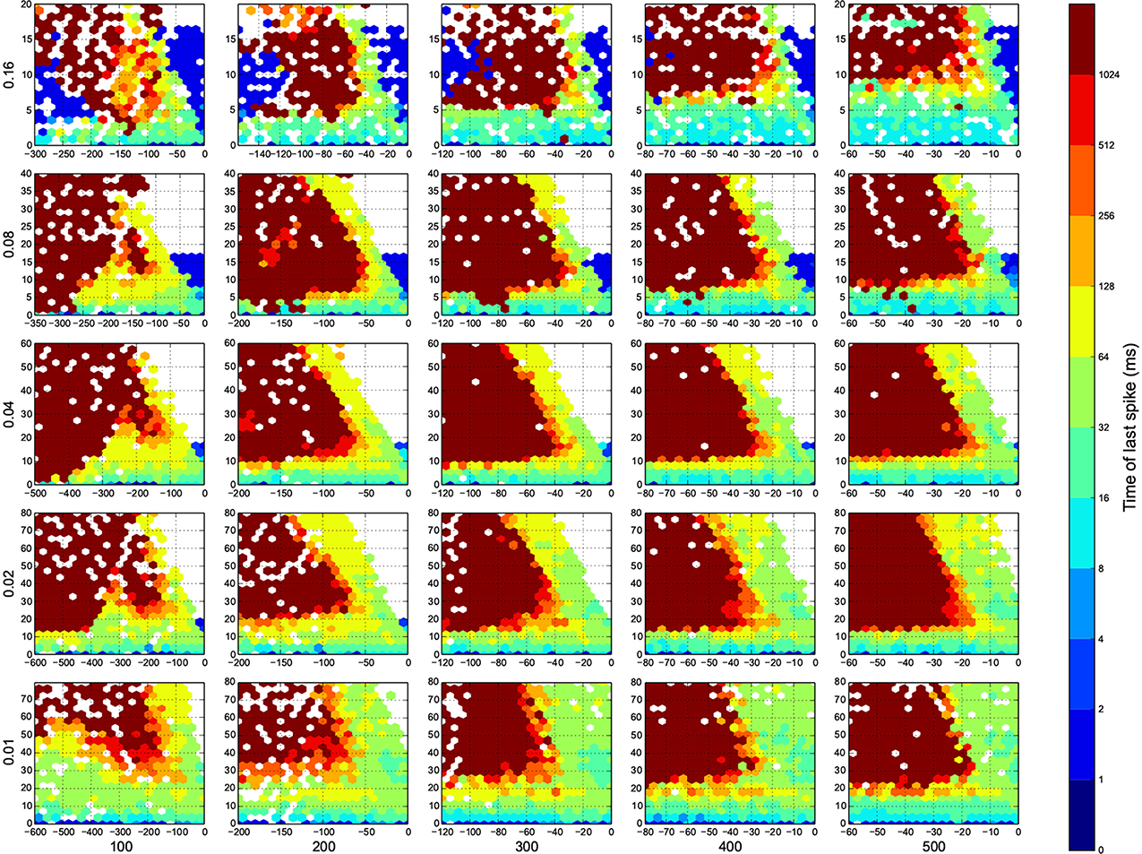
Figure 6. The time of last spike in each trial. Dark red means the simulation ended before the network returns to its resting state. Here white means there was not any simulation data at that bin, or all the data were unreliable. The information are arranged according to the template of Figure 3.

FIGURE 7

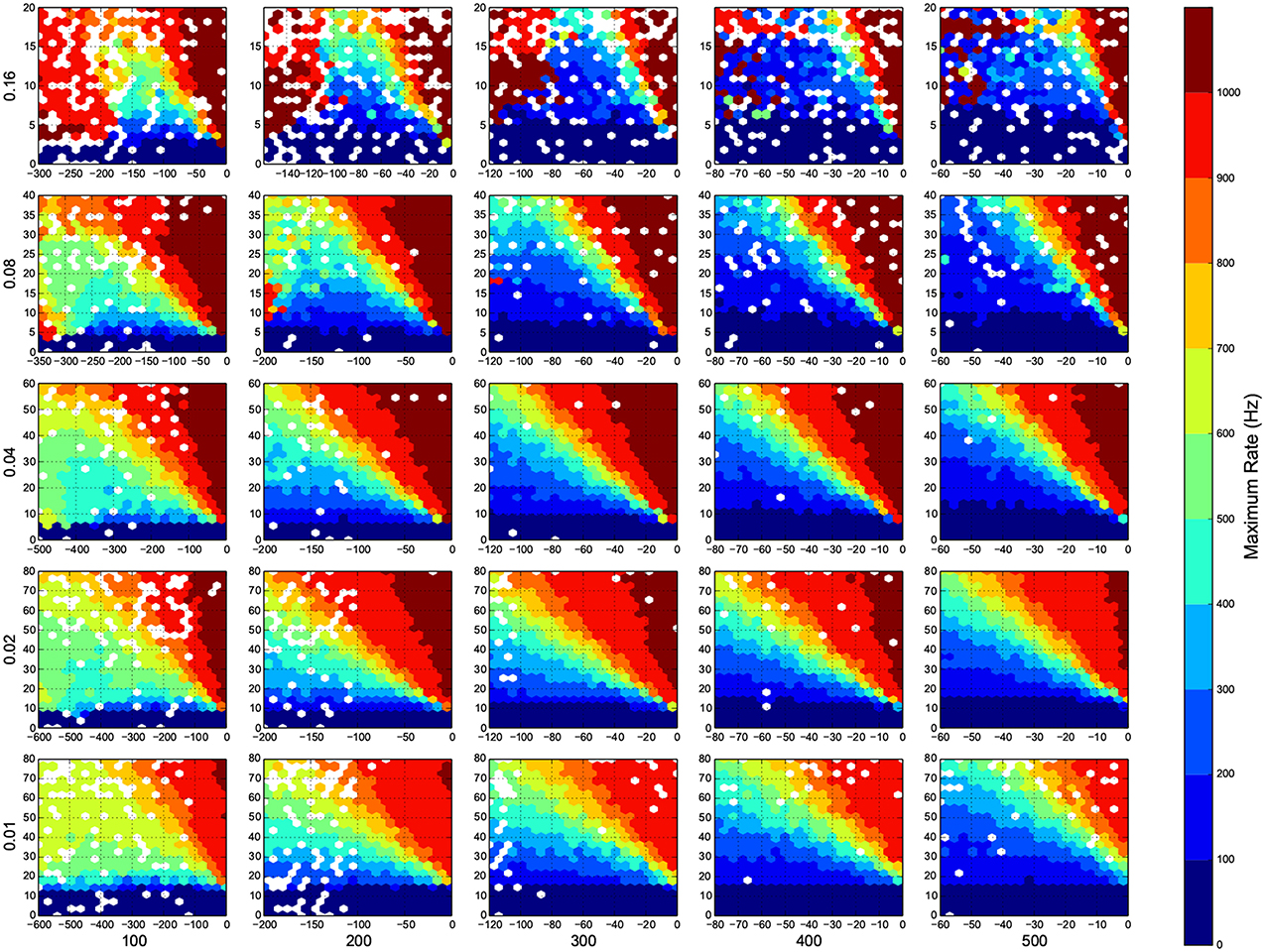
Figure 7. Maximum firing rate in each trial. Here white means there was not any simulation data at that bin. The information are arranged according to the template of Figure 3.

FIGURE 8

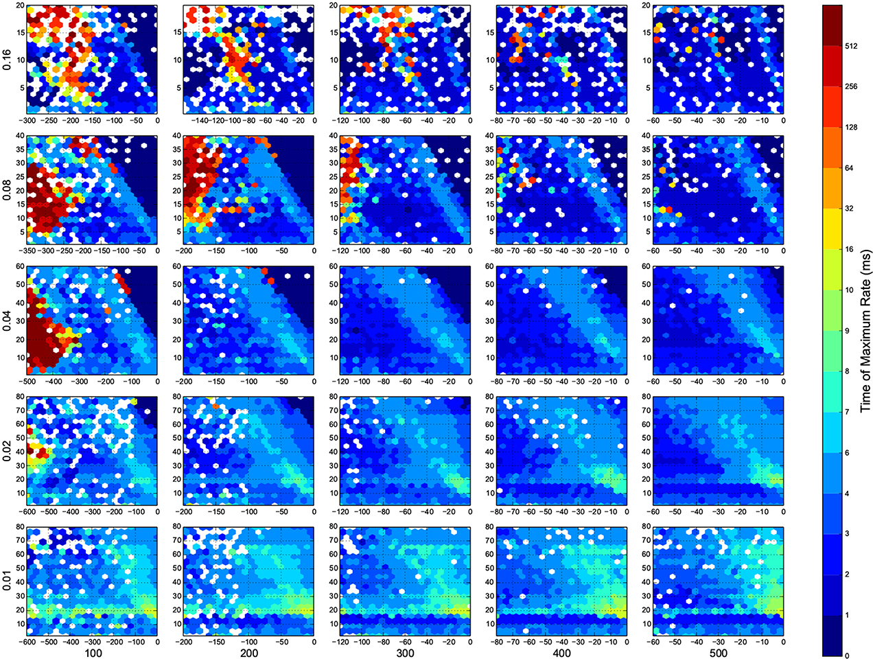
Figure 8. The time that maximum firing rate happens in each trial. Here white means there was not any simulation data at that bin. The information are arranged according to the template of Figure 3.

4. Discussion

In Figure 4, top right corner of each figure is empty (white). This is where the excitatory neurons dominates and the network riches its maximum firing rate, this region is visible in Figure 7 as the darkest shade of red. The lesft side of each graph, where the inhibitory subnetwork dominates, is also empty, but this time because networks did not return to resting states. More detail about the length of activity demonstrated in Figure 6.

A narrow band seperate this two regins, on this band, the inhibitory and excitatory network are balancing out each other. As we increase the number of connections, this band gets narrower, the delicate balance can be easily disturbed. The dynamic ranges on this band is low or moderate.

At the bottom of each graph, there is another region with valid data points. In this region, excitatory sub networks are not strong enough to saturate the system, so we have a good dynamic range regardless of the inhibitory synaptic weights. Nevertheles, stronger inhibitory sub networks improves the dynamic range.

For the calculation of dynamic range, only trials who returned to resting state have been used. But in many other trials the network sustained its activity upto the very last miliscond of simulation (Figure 6). These networks shows interesting oscillatory behaviures, that can be seen in Figures 5, 9. The oscillations are mostly α and β waves, with fewer case of γ waves. There are also δ and θ waves, but the simulation time of 1 s may not be enough to study these waves.

FIGURE 9

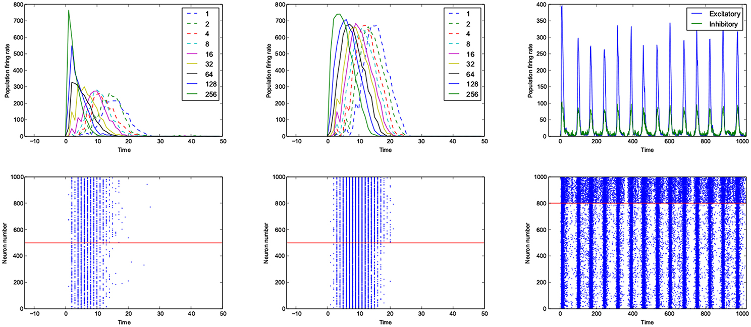
Figure 9. An example of fast respoding network with a good dynamic range (left), poor dynamic range (middle) and an example of oscillatory network (right). Population rates as a function of time (top). The spiking avtivity of neurons (bottom). The red line seperates excitatory neurons (below the line) from inhibitory neurons (above the line).

The networks are stimulated with only a pulse, and then they are left alone, even though there is not any spontaneous activity implemented in the model, yet, the networks show sustained oscillations.

The oscillation are mostly β-waves, and they happen in the region of dominating inhibitory sub networks. As we get to the balanced inhibitory-excitatory band, the oscillations become α-waves.

It seems that the results are not very sensitive to the parameters, We can have good dynamic range over some value of parameters, and we can have neural oscillators in different settings. These finding agrees with Prinz et al. (2004); Marder et al. (2007); Marder and Taylor (2011); Marder (2011); Gutierrez et al. (2013).

The results of this paper, specially Figures 4, 5, serves as a starting point to decide about parameters in a neural simulation, and they may help to find the networks with desired behavior.

This work by no mean is complete, I only studied the effect of four parameters, in just one model, over dynamic range and oscillations. Many other parameters could be included, like synaptic delay and distribution of weights or connections. Also it is interesting to know if my results holds for simpler models, like Integrate-and-fire.

At the end I suggest that any numerical simulation of neural network should be accompanied with such a phase diagram, it demonstrate the robustness of the results in respect to the parameters. One good example is the the work of Roy et al. (2013), where they made such diagram to compare experimental data of orientation selectivity index of mouse primary virtual cortex to their model.

Conflict of Interest Statement

The author declares that the research was conducted in the absence of any commercial or financial relationships that could be construed as a potential conflict of interest.

Acknowledgment

The research presented in this paper was carried out on the High Performance Computing Cluster supported by the Computer Science department of Institute for Research in Fundamental Sciences (IPM).

Supplementary Material

The Supplementary Material for this article can be found online at: “http://www.frontiersin.org/journal/10.3389/fncom.2015.00019/abstract.”

References

Akam, T., and Kullmann, D. M. (2010). Oscillations and filtering networks support flexible routing of information. Neuron 67, 308–320. doi: 10.1016/j.neuron.2010.06.019

Pubmed Abstract | Pubmed Full Text | CrossRef Full Text | Google Scholar

Attwell, D., and Laughlin, S. B. (2001). An energy budget for signaling in the grey matter of the brain. J. Cereb. Blood Flow Metab. 21, 1133–1145. doi: 10.1097/00004647-200110000-00001

Pubmed Abstract | Pubmed Full Text | CrossRef Full Text | Google Scholar

Augustin, M., Ladenbauer, J., and Obermayer, K. (2013). How adaptation shapes spike rate oscillations in recurrent neuronal networks. Front. Comput. Neurosci. 7:9. doi: 10.3389/fncom.2013.00009

CrossRef Full Text | Google Scholar

Bakhtiari, R., Mohammadi Sephavand, N., Nili Ahmadabadi, M., Nadjar Araabi, B., and Esteky, H. (2012). Computational model of excitatory/inhibitory ratio imbalance role in attention deficit disorders. J. Comput. Neurosci. 33, 389–404. doi: 10.1007/s10827-012-0391-y

Pubmed Abstract | Pubmed Full Text | CrossRef Full Text | Google Scholar

Barbour, B., Brunel, N., Hakim, V., and Nadal, J.-P. (2007). What can we learn from synaptic weight distributions? Trends Neurosci. 30, 622–629. doi: 10.1016/j.tins.2007.09.005

Pubmed Abstract | Pubmed Full Text | CrossRef Full Text | Google Scholar

Binzegger, T., Douglas, R. J., and Martin, K. A. C. (2004). A quantitative map of the circuit of cat primary visual cortex. J. Neurosci. 24, 8441–8453. doi: 10.1523/JNEUROSCI.1400-04.2004

Pubmed Abstract | Pubmed Full Text | CrossRef Full Text | Google Scholar

Brette, R., Rudolph, M., Carnevale, T., Hines, M., Beeman, D., Bower, J. M., et al. (2007). Simulation of networks of spiking neurons: a review of tools and strategies. J. Comput. Neurosci. 23, 349–398. doi: 10.1007/s10827-007-0038-6

Pubmed Abstract | Pubmed Full Text | CrossRef Full Text | Google Scholar

Brown, S. P., and Hestrin, S. (2009). Intracortical circuits of pyramidal neurons reflect their long-range axonal targets. Nature 457, 1133–1136. doi: 10.1038/nature07658

Pubmed Abstract | Pubmed Full Text | CrossRef Full Text | Google Scholar

Buice, M. A., and Cowan, J. D. (2009). Statistical mechanics of the neocortex. Prog. Biophys. Mol. Biol. 99, 53–86. doi: 10.1016/j.pbiomolbio.2009.07.003

Pubmed Abstract | Pubmed Full Text | CrossRef Full Text | Google Scholar

Chklovskii, D., Schikorski, T., and Stevens, C. (2002). Wiring optimization in cortical circuits. Neuron 34, 341–347. doi: 10.1016/S0896-6273(02)00679-7

Pubmed Abstract | Pubmed Full Text | CrossRef Full Text | Google Scholar

Dayan, P., and Abbott, L. (2001). Theoretical Neuroscience: Computational and Mathematical Modeling of Neural Systems. Cambridge, MA: MIT Press.

Google Scholar

Erds, P., and Rényi, A. (1960). On the evolution of random graphs. Publ. Math. Inst. Hungar. Acad. Sci. 5, 17–61.

Google Scholar

Feldmeyer, D. (2012). Excitatory neuronal connectivity in the barrel cortex. Front. Neuroanat. 6:24. doi: 10.3389/fnana.2012.00024

Pubmed Abstract | Pubmed Full Text | CrossRef Full Text | Google Scholar

Fidjeland, A. K., and Shanahan, M. P. (2010). “Accelerated simulation of spiking neural networks using GPUs,” in The 2010 International Joint Conference on Neural Networks (IJCNN) (Barcelona), 1–8.

Google Scholar

Fidjeland, A. K., Roesch, E. B., Shanahan, M. P., and Luk, W. (2009). “NeMo: a platform for neural modelling of spiking neurons using GPUs,” in 2009 20th IEEE International Conference on Application-specific Systems, Architectures and Processors (Boston, MA), 137–144.

Google Scholar

Goodman, D., and Brette, R. (2008). Brian: a simulator for spiking neural networks in python. Front. Neuroinform. 2:5. doi: 10.3389/neuro.11.005.2008

Pubmed Abstract | Pubmed Full Text | CrossRef Full Text | Google Scholar

Gutierrez, G. J., O'Leary, T., and Marder, E. (2013). Multiple mechanisms switch an electrically coupled, synaptically inhibited Neuron between competing rhythmic oscillators. Neuron 77, 845–858. doi: 10.1016/j.neuron.2013.01.016

CrossRef Full Text | Google Scholar

Herz, A. V. M., Gollisch, T., Machens, C. K., and Jaeger, D. (2006). Modeling single-neuron dynamics and computations: a balance of detail and abstraction. Science 314, 80–85. doi: 10.1126/science.1127240

Pubmed Abstract | Pubmed Full Text | CrossRef Full Text | Google Scholar

Izhikevich, E. M. (2003). Simple model of spiking Neurons. IEEE Trans. Neural Netw. 14, 1569–1572. doi: 10.1109/TNN.2003.820440

Pubmed Abstract | Pubmed Full Text | CrossRef Full Text | Google Scholar

Izhikevich, E. M. (2004). Which model to use for cortical spiking neurons? IEEE Trans. Neural Netw. 15, 1063–1070. doi: 10.1109/TNN.2004.832719

Pubmed Abstract | Pubmed Full Text | CrossRef Full Text | Google Scholar

Ko, H., Hofer, S. B., Pichler, B., Buchanan, K. A., Sjöström, P. J., and Mrsic-Flogel, T. D. (2011). Functional specificity of local synaptic connections in neocortical networks. Nature 473, 87–91. doi: 10.1038/nature09880

CrossRef Full Text | Google Scholar

Lefort, S., Tomm, C., Floyd Sarria, J.-C., and Petersen, C. C. H. (2009). The excitatory neuronal network of the C2 barrel column in mouse primary somatosensory cortex. Neuron 61, 301–316. doi: 10.1016/j.neuron.2008.12.020

Pubmed Abstract | Pubmed Full Text | CrossRef Full Text | Google Scholar

Lim, D. H., Mohajerani, M. H., Ledue, J., Boyd, J., Chen, S., and Murphy, T. H. (2012). In vivo large-scale cortical mapping using channelrhodopsin-2 stimulation in transgenic mice reveals asymmetric and reciprocal relationships between cortical areas. Front. Neural Circuits 6:11. doi: 10.3389/fncir.2012.00011

CrossRef Full Text | Google Scholar

Liu, X., Ramirez, S., Pang, P. T., Puryear, C. B., Govindarajan, A., Deisseroth, K., et al. (2012). Optogenetic stimulation of a hippocampal engram activates fear memory recall. Nature 484, 381–385. doi: 10.1038/nature11028

Pubmed Abstract | Pubmed Full Text | CrossRef Full Text | Google Scholar

Marder, E., and Taylor, A. L. (2011). Multiple models to capture the variability in biological neurons and networks. Nat. Neurosci. 14, 133–138. doi: 10.1038/nn.2735

Pubmed Abstract | Pubmed Full Text | CrossRef Full Text | Google Scholar

Marder, E., Tobin, A.-E., and Grashow, R. (2007). How tightly tuned are network parameters? Insight from computational and experimental studies in small rhythmic motor networks. Prog. Brain Res. 165, 193–200. doi: 10.1016/S0079-6123(06)65012-7

Pubmed Abstract | Pubmed Full Text | CrossRef Full Text | Google Scholar

Marder, E. (2011). Variability, compensation, and modulation in neurons and circuits. Proc. Natl. Acad. Sci. U.S.A. 108(Suppl.), 15542–15548. doi: 10.1073/pnas.1010674108

Pubmed Abstract | Pubmed Full Text | CrossRef Full Text | Google Scholar

McNally, L., Brown, S. P., and Jackson, A. L. (2012). Cooperation and the evolution of intelligence. Proc. R. Soc. B Biol. Sci. 279, 3027–3034. doi: 10.1098/rspb.2012.0206

CrossRef Full Text | Google Scholar

Mejias, J., and Longtin, A. (2012). Optimal heterogeneity for coding in spiking neural networks. Phys. Rev. Lett. 108, 1–5. doi: 10.1103/PhysRevLett.108.228102

Pubmed Abstract | Pubmed Full Text | CrossRef Full Text | Google Scholar

Nicholls, J. G., Martin, A. R., Fuchs, P. A., Brown, D. A., Diamond, M. E., and Weisblat, D. A. (2012). From Neuron to Brain, 5th Edn. Sunderland, MA: Sinauer Associates.

Google Scholar

Niven, J. E., and Laughlin, S. B. (2008). Energy limitation as a selective pressure on the evolution of sensory systems. J. Exp. Biol. 211(Pt 11), 1792–1804. doi: 10.1242/jeb.017574

Pubmed Abstract | Pubmed Full Text | CrossRef Full Text | Google Scholar

Perin, R., Berger, T. K., and Markram, H. (2011). A synaptic organizing principle for cortical neuronal groups. Proc. Natl. Acad. Sci. U.S.A. 108, 5419–5424. doi: 10.1073/pnas.1016051108

Pubmed Abstract | Pubmed Full Text | CrossRef Full Text | Google Scholar

Peron, S., and Svoboda, K. (2011). From cudgel to scalpel: toward precise neural control with optogenetics. Nat. Methods 8, 30–34. doi: 10.1038/nmeth.f.325

Pubmed Abstract | Pubmed Full Text | CrossRef Full Text | Google Scholar

Prinz, A. A., Bucher, D., and Marder, E. (2004). Similar network activity from disparate circuit parameters. Nat. Neurosci. 7, 1345–1352. doi: 10.1038/nn1352

Pubmed Abstract | Pubmed Full Text | CrossRef Full Text | Google Scholar

Roy, D., Tjandra, Y., Mergenthaler, K., Petravicz, J., Runyan, C. A., Wilson, N. R., et al. (2013). Afferent Specificity, Feature Specific Connectivity Influence Orientation Selectivity: A Computational Study in Mouse Primary Visual Cortex. Available online at: http://arxiv.org/abs/1301.0996

Song, S., Miller, K. D., and Abbott, L. F. (2000). Competitive hebbian learning through spike-timing-dependent synaptic plasticity. Nat. Neurosci. 3, 919–926. doi: 10.1038/78829

Pubmed Abstract | Pubmed Full Text | CrossRef Full Text | Google Scholar

Sterratt, D., Graham, B., and Gillies, A. (2011). Principles of Computational Modelling in Neuroscience. Cambridge: Cambridge University Press

Google Scholar

Toettcher, J. E., Voigt, C. A., Weiner, O. D., and Lim, W. A. (2011). The promise of optogenetics in cell biology: interrogating molecular circuits in space and time. Nat. Methods 8, 35–38. doi: 10.1038/nmeth.f.326

CrossRef Full Text | Google Scholar