Segmental Bayesian estimation of gap-junctional and inhibitory conductance of inferior olive neurons from spike trains with complicated dynamics

1. Introduction

Rapid progress in computer science now enables simulations of neuronal networks with high complexity. Advanced technology in neuroscience—such as the multiple electrode arrays, optical recording using various dyes, and optogenetic techniques—enable sampling of a massive amount of neuronal data from the brain (Nikolenko et al., 2007; Pastrana, 2010). Combining technologies across two fields of science to understand the computations in the brain still face severe difficulties mainly because of the fact that the technologies of both fields are still rather simplistic compared to a huge complexity of the brain network. It is nevertheless a big challenge in computational neuroscience to construct a brain model that simulates brain computations.

Modeling of the brain requires a number of parameters that are difficult to measure using current technology. Various approaches have been developed to resolve this “parameter estimation” problem. There are deterministic approaches that find unique solutions by optimization techniques, including the conjugate gradient, genetic algorithm, simulated annealing, and random search methods (Kirkpatrick et al., 1983; Vanier and Bower, 1999; Keren et al., 2005). These methods are only applicable in relatively well-defined environments where the complexity of the system—such as the hierarchy, granularity, and degrees-of-freedom—is comparable between the model and experiment. Otherwise, parameter estimation problems become ill-posed. Another deterministic approach uses state and parameter reconstruction based on rather simplified neural models, such as Hindmarsh–Rose and FitzHugh–Nagumo models (Fairhurst et al., 2010; Tyukin et al., 2010). Stochastic approaches were developed to overcome these difficulties, e.g., Markov random field model that estimates membrane resistance from the optical imaging data (Kitazono et al., 2012) and stochastic models that estimate the synaptic conductance from the electrophysiological recording data (Berg and Ditlevsen, 2013). Nonlinear state space modeling has also been applied to estimate hidden dynamical variables as well as unknown parameters from the optical recording data (Tsunoda et al., 2010; Meng et al., 2011). These approaches were also limited to the cases of a small mismatch between the model and experiment where the system complexity for the two cases was almost comparable. Another difficulty is that brain dynamics are non-stationary. Neuronal firing in the brain exhibits various types of irregularity in its dynamics (Ikeda et al., 1989; Kaneko, 1990; Tsuda, 1992; Tsuda et al., 2004) that are difficult to model.

The present study aims to estimate the conductance of the inferior olive (IO) neurons from spike train data using the network model simulation, which is confronted by various mismatch problems in the system complexity between the model and experimental data. The first is the granularity-hierarchy mismatch. The experimental spike data are generated by the network while the parameters to be estimated exist at the synapses. The second is the degrees of freedom mismatch. The real IO conveys far more complicated structures with huge degrees of freedom than those for the model, the number of IO neurons being at least four orders of magnitude greater than that for the model. The third mismatch is that IO firing dynamics are highly non-stationary, showing chaos, oscillations and other non-stationary properties (Schweighofer et al., 2004), while those of the model convey rather low non-stationarity. Therefore, we cannot expect that the network model can perfectly simulate the experimental data, and no one-to-one mapping would hold between the experimental data and the model parameters. None of the current approaches, either deterministic or stochastic, would be suitable for resolving this huge mismatch problem.

A previous study (Onizuka et al., 2013) resolved this huge mismatch problem by combining the deterministic approach with the statistical one in two ways. First, the model parameters to be fitted to the experimental data were estimated in a deterministic fashion as those of simulation data with the minimum distance to the experimental ones. Nevertheless, this procedure can be regarded as an extreme case of a class of statistical Bayesian estimation algorithms where a variance of a mixture-of-Gaussian model to translate spike data to the parameter values is assumed to be infinitely small. Second, the experimental spike data for every neuron were divided into short segments and the parameters were estimated for each segment. Then, these parameter values were pooled to give the probability distribution of the parameter values for the entire neuronal data, thus introducing the statistical estimates. The aim of the current study is to present a general framework based on a hierarchical Bayesian inference, adopting the same estimation problem of the two conductance values in IO network as used in our previous study. Our method estimates conductance values for spike segments using the forward models generalized to the entire spike data and merges the segmental estimates into a single estimate for every neuron. The segmental Bayes is equivalent to the method used in the recent studies that introduced the system noise in order to reduce the estimation errors due to modeling errors (Arridge et al., 2006; Huttunen and Kaipio, 2007; Kaipio and Somersalo, 2007). To allow segmental fluctuations in the parameter estimates and to merge the estimates for a single neuron imply to assume noise for parameter estimation with the constraint to minimize fluctuations within single neurons. This neuronal constraint avoids over-fitting of the forward models to experimental data that was the case in the previous study, reducing the number of Gaussians by three orders of magnitude, and the fitting errors to less than one-third of those in previous studies with highly non-stationary data.

2. Methods

2.1. Experimental Data

We used the same spike data as those for a previous study (Onizuka et al., 2013). They include the spike data collected from two picrotoxin (PIX; Lang et al., 1996; Lang, 2002) and one carbenoxolone (CBX; Blenkinsop and Lang, 2006) studies. These studies sampled the IO spike as the complex spikes of Purkinje cells and blocked the inhibitory and gap-junctional conductance (g_i and g_c) of IO neuronal circuitry by application of PIX and CBX. PIX and CBX experiments contained the spike data of 500-s-long samples from 136 and 35 neurons, respectively.

2.2. Conductance Parameters Estimation

It has been shown that the inhibitory synaptic conductance (g_i) and the gap-junction conductance (g_c) are the two major determinants of the IO firing (Llinas et al., 1974; Llinas and Yarom, 1981; Best and Regehr, 2009). Our goal was to inversely estimate these conductance values from the IO firing data.

This inverse problem contains two practical difficulties. One is that it is an ill-posed problem because of the fact that IO firing dynamic depends on the ratio of g_i and g_c rather than their actual values and the other is because of the highly non-stationary and complicated firing dynamics that are difficult for current IO network models to precisely simulate. To overcome these difficulties, we tested a segmental Bayesian method.

The first difficulty is resolved by introducing a neuronal commonality constraint such that g_c remains unchanged between PIX and control (CON) conditions, whereas g_i remains unchanged between CBX and CON conditions in one neuron. The second difficulty was resolved by dividing whole spike trains into short time segments, estimating the parameters in each segment, and then integrating them into a single value according to hierarchical Bayesian inference.

In the segmental Bayesian method, the following six steps were applied to each neuron's data (EXP) to estimate the conductance values (g_i, g_c) of each neuron:

1. The network of IO neurons is simulated to generate spike trains (SIM data).

2. We evaluated the IO firing dynamics in short time segments in terms of a feature vector (FV) composed of multiple quantities such as mean firing rate, auto- and cross-correlation, local variation (LV), minimal distances (MDs), and spike distance (SD).

3. We transformed the FVs into low dimensional principal components according to feature extraction based on mutual information and principal component analysis (PCA).

4. The likelihood function was estimated as a forward model using the Gaussian mixture model in PCA space based on the SIM data.

5. The likelihood of EXP data for segments was calculated.

6. Finally, single g_i and g_c values for the whole experimental data in one neuron was estimated by a hierarchical Bayesian inference, where a neuronal commonality constraint was imposed as a hierarchical prior and the variability of g_i and g_c in segments was represented as the model variance.

2.2.1. IO neuronal network simulation

The model was composed of 3×3 neurons (Figure 1C), each of which consists of a soma, dendrite, and spine compartments (Figure 1A). The neurons were connected to each other via gap-junctions (Figure 1B). We simulated the IO firing according to the equations representing the equivalent circuitry summarized in Figures 1A–C (cf. Equations A1–A17, Onizuka et al., 2013).

FIGURE 1

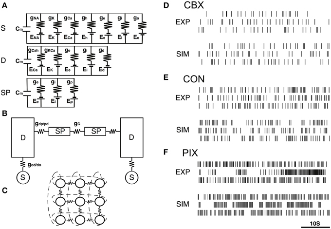
Figure 1. IO network model and representatives of EXP and SIM spike trains. (A–C) A schematic diagram of the IO network model consisting of 9 neurons, each of which consists of the soma (S), dendrite (D) and spine compartments (SP). The S, D, and SP compartments contain five, three, and one ionic channels defined by the modified Hodgkin–Huxley equations (cf. Equations A1–A17, Onizuka et al., 2013) and the excitatory and inhibitory input conductance (g_e and g_i). Two neighboring neurons are coupled via gap junctional conductance (g_c) and axial spine conductance (g_dp/pd). (D–F) Three representative pairs of EXP and SIM spike segment (50 s) that showed the closest match in the 3D PCA space constructed of the 25 FVs for the CBX, CON, and PIX conditions. EXP spike segments in each condition are of different neurons.

The soma, dendrite and spine compartments received the excitatory and inhibitory inputs through 10, 80, and 10 synapses, respectively, driven by Gaussian noise generators. Synaptic noise was used to produce spatiotemporal dynamics in the simulation spike trains. We found that the length used for the simulation data in the previous study (500 s) was insufficient to cover the spatio-temporal dynamics of the IO spike data (cf. Figures 3A–C), and therefore generated 10× longer (e.g, 5000 s) simulation data.

Several studies have shown that IO neurons covey heterogeneity in their membrane conductance (Manor et al., 1997; Hoge et al., 2011; Torben-Nielsen et al., 2012). We assumed comparable variations of g_Cal and g_c, in our model, sampling them from uniform distributions with the maximum deviation set at 5% of the mean. The two parameters of concern, g_i and g_c, were varied in the range of [0–1.5 mS/cm²] and [0–2.0 mS/cm²], respectively, with an increment of 0.05 mS/cm², whereas the excitatory conductance g_e was fixed at 0.03 mS/cm².

2.2.2. Feature Vectors

We also used the same FVs as those in a previous study adding the spike distance metric (Kreuz et al., 2013) to characterize the spatiotemporal properties of the spike train (cf. Methods, Onizuka et al., 2013). To perform the segmental Bayesian inference, we divided the experimental spike data into 10 50-s segments. For each segment, 68 features were evaluated and they were averaged across three neurons to improve the signal-to-noise ratio. The first three classes of the FV represent temporal properties, while the last three represent spatial properties of the firing patterns.

1. The mean firing rate (FR) of spike segments was calculated as the number of spikes in 1 s.

2. The local variation (LV) was calculated as

$\begin{array}{cc}LV=\frac{1}{R-1}{\displaystyle \sum _{r=1}^{R-1}\frac{3{(T_{r+1}-T_r)}^2}{{(T_{r+1}+T_r)}^2}}& \left(1\right)\end{array}$

where T_r (r = 1, 2…R) is the r-th inter-spike interval (ISI) (Shinomoto et al., 2005).

3. The auto-correlogram for 20 delays (ACG 1–20) ranged from 0 to 1000 ms with a bin size of 50 ms.

$\begin{array}{cc}AC{G}_{x,i}(\tau )={\displaystyle \sum _{k=1}^K{x}_i}(t_k)x_i(t_k-\tau )& \left(2\right)\end{array}$

where x_i(t_k) represents the occurrence of spikes at the k-th time step in i-th neuron and τ is the time delay.

4. The cross-correlogram for 20 delays (CCG 1–20) corresponding to delays of 0–50 ms, 50–100 ms, …c 950–1000 ms were computed as:

$\begin{array}{cc}CC{G}_{x,i,j}(\tau )={\displaystyle \sum _{k=1}^K{x}_i}(t_k)x_j(t_k-\tau )& \left(3\right)\end{array}$

5. The minimal distance (Hirata and Aihara, 2009) (MD1–25) was defined as a normalized distribution of

$\begin{array}{cc}{s}_l^{i,j}=1-\exp \left(\frac{-2{\min }_m|t_l^i-t_m^j|}{{\overline{d}}_j}\right)& \left(4\right)\end{array}$

between the l-th spike of neuron i and a spike of neuron j. Here, t_lⁱ is the time of l-th spike of the neuron i, d_j is the mean ISI of the j-th neuron, and m ranged from 1 to the total number of spikes of neuron j. If the spike train is generated by a random process, the distribution will be uniformly distributed between 0 and 1.

6. The spike distance (Kreuz et al., 2013) (SD) was defined as

$\begin{array}{cc}{D}_S=\frac{1}{T}{\displaystyle {\int }_{t=0}^{T}S}(t)\text{d}t& \left(5\right)\end{array}$

where S(t) are instantaneous dissimilarity values derived from differences between the spike times of the two spike trains and T is the recording time. SD is bounded in the range [0, 1] with the value zero obtained for perfectly identical spike trains.

2.2.3. Mutual Information and Feature Extraction

As described in Section 2.2.2, a total of 68 features were computed from the firing data. To estimate the conductance parameters efficiently, only the main features that contain rich information on g_i and g_c were extracted from the FV according to the mutual information (MI) between the FV and the conductance values.

We let g = (g_i, g_c) ∈ G as a pair of the conductance parameters and x ∈ X denote one component of the FV. Then, the MI that represents the amount of information of G conveyed by x was computed as:

$\begin{array}{cc}\begin{array}{l}I(G;x)={\displaystyle \sum _{g\in G}P}(x,g)\log \left(\frac{P(x,g)}{P(x)P(g)}\right)\\ ={\displaystyle \sum _{g\in G}P}(x|g)P(g)\log \left(\frac{P(x|g)}{P(x)}\right)\end{array}& \left(6\right)\end{array}$

Here, the conditional distribution P(x|g) was approximated as a histogram of x given a pair of (g_i, g_c), the distribution P(x) was assumed to be a histogram of x, and P(g) was assumed to be a uniform distribution. The 68 FVs were rated by the MI and top 25 FVs were selected for principal component analysis.

2.2.4. Principal Component Feature Vectors

To reduce the redundancy further, principal component analysis (PCA) was conducted as a solution to the following equation:

$\begin{array}{cc}(X^{T}X)W=\lambda W,& \left(7\right)\end{array}$

where (X^T X) is the covariance matrix of the 25 features of EXP spike data X. We used a Statistical Toolbox (MATLAB^®) to calculate the eigenvector W and eigenvalues λ. The principal component vector Y was computed as the linear transformation of the feature vector X as follows:

$\begin{array}{cc}Y=XW& \left(8\right)\end{array}$

Finally, the top three principal components of Y were selected according to the highest eigenvalues (0.27, 0.21 and 0.09) for construction of the forward model.

2.2.5. Forward Model

To evaluate the fitting between the experimental and simulation data, we constructed a forward model as a likelihood function in PCA space using the simulation data. The likelihood functions at each grid point of g = (g_i, g_c) were approximated by Gaussian mixture models:

$\begin{array}{cc}P(y|g)={\displaystyle \sum _{k=1}^K{\pi }_k}N({\mu }_k,{\Sigma }_k),& \left(9\right)\end{array}$

where N(μ, Σ) is the multivariate Normal (Gaussian) distribution with mean μ and covariance Σ. The number of components K, mixing coefficients π_k, means μ_k and covariance matrices Σ_k of Gaussian mixtures were estimated from the simulated data for a given parameter set g using the variational Bayes algorithm (Sato, 2001; Chapter 9 of Bishop, 2006). The average number of component K, which was automatically determined by the algorithm, was 8.55. The performance of the fitting was confirmed by comparing the PC scores of SIM with that predicted by the forward model by the statistical energy test (Aslan and Zech, 2005).

2.2.6. Segment-Wise Neuronal Bayesian Model

Given the principal component features y as described in Section 2.2.4 (Equation 8), we needed to estimate the conductance parameters g_i and g_c that generated the corresponding firing dynamics of the IO neurons. Our model can be considered as a kind of hierarchical Bayesian model (Chapter 5 of Gelman et al., 2013), which consists of three probability distributions: the likelihood function, prior distribution and hyper-prior distribution. The likelihood function was obtained as shown in Section 2.2.5. The prior and hyper-prior distributions function as the constraints for the Bayesian estimation. The model parameters were finally estimated by computing the posterior distribution and the model evidence.

• Bayesian model with the commonality constraint

First, a commonality constraint was introduced based on the fact that PIX and CBX selectively reduce g_i and g_c, respectively. This implies that g_c remains unchanged between the PIX and CON conditions, whereas g_i remains unchanged between the CBX and CON conditions. The commonality constraint thus assumes that PIX and CON data share the same conductance value for g_c in a prior distribution, while CBX and CON data share the same g_i.

We let y^CON(t) and y^CON = [y^CON(1), y^CON(2), …, y^CON(T)] denote the feature vector for time segment t and the collection of the segment-wise feature vectors for the control conditions, respectively. Similarly y^pha(t) and y^pha were defined for the pharmacological condition, where pha stands for either PIX or CBX. In addition, we let [g^CON_i, g^CON_c, g^pha_i, g^pha_c] denote the conductance parameters for a neuron under the control and pharmacological conditions.

Thus, the likelihood function of the model is

$\begin{array}{cc}\begin{array}{l}P\left(y^{CON},y^{pha}|g_i^{CON},g_c^{CON},g_i^{pha},g_c^{pha}\right)\\ =P\left(y^{CON}|g_i^{CON},g_c^{CON}\right)P\left(y^{pha}|g_i^{pha},g_c^{pha}\right)\\ ={\displaystyle \prod _{t}P}\left(y^{CON}(t)|g_i^{CON},g_c^{CON}\right)P\left(y^{pha}(t)|g_i^{pha},g_c^{pha}\right),\end{array}& \left(10\right)\end{array}$

where P(y|g_i, g_c) is the probability density function constructed from the forward model. As prior distributions, we assume uniform distributions for g_i and g_c with commonality constraints. In the case of pha = PIX, g^CON_c = g^PIX_c, thus

$\begin{array}{cc}\begin{array}{l}{P}_0\left(g_i^{CON},g_c^{CON},g_i^{pha},g_c^{pha}\right)\\ =P_0\left(g_i^{CON},g_i^{PIX},g_c^{CON}\right)\delta \left(g_c^{CON}-g_c^{PIX}\right)\propto \delta \left(g_c^{CON}-g_c^{PIX}\right)\end{array}& \left(11\right)\end{array}$

where δ (g_c) is the Dirac delta function. In the case of pha = CBX

$\begin{array}{cc}\begin{array}{l}{P}_0\left(g_i^{CON},g_c^{CON},g_i^{pha},g_c^{pha}\right)\\ =P_0\left(g_c^{CON},g_c^{CBX},g_i^{CON}\right)\delta \left(g_i^{CON}-g_i^{CBX}\right)\propto \delta \left(g_i^{CON}-g_i^{CBX}\right)\end{array}& \left(12\right)\end{array}$

Equations (10), (11) or (10), (12) constituted the neuronal Bayesian model.

• Hierarchical Bayesian model with the neuronal and commonality constraints

In addition to the commonality constraint, a neuronal constraint was introduced. This constraint dealt with the estimation errors caused by the non-stationarity of the IO dynamics as well as by the incapability of the model to faithfully reproduce the complicated firing patterns of the experimental data. To minimize such errors, we divided the spike data of each neuron into segments, applied the above Bayesian model to estimate g_i and g_c for every segment, and then merged the segmental estimates into a single estimate for each neuron. In this framework, the estimation errors from non-stationarity can be treated as the variance of the estimates.

This idea can be implemented by expanding the Bayesian model to a hierarchical one that employs an additional hierarchical prior distribution for merging the segmental estimates. In this model, each segment of data is generated from a segment-wise conductance parameters [g^CON_i(t), g^CON_c(t), g^pha_i(t), g^pha_c(t)] which vary around neuronal conductance parameters [g^CON_i, g^CON_c, g^pha_i, g^pha_c]. The variations in the conductance parameters are considered to reflect discrepancies between the simulation dynamics and the complex dynamics of real neurons.

Thus, the likelihood function became

$\begin{array}{cc}\begin{array}{l}P\left(y^{CON},y^{pha}|g_i^{CON}(1:T),g_c^{CON}(1:T),g_i^{pha}(1:T),g_c^{pha}(1:T)\right)\\ =P\left(y^{CON}|g_i^{CON}(1:T),g_c^{CON}(1:T)\right)P\left(y^{pha}|g_i^{pha}(1:T),g_c^{pha}(1:T)\right)\\ ={\displaystyle \prod _{t}P}\left(y^{CON}(t)|g_i^{CON}(t),g_c^{CON}(t)\right)P\left(y^{pha}(t)|g_i^{pha}(t),g_c^{pha}(t)\right),\end{array}& \left(13\right)\end{array}$

where g^CON_i(1 : T) = [g^CON_i(1), g^CON_i(2), …, g^CON_i (T)] are collections of the segment-wise conductance, and similarly, for g^CON_c(1 : T), g^pha_i(1 : T) and g^pha_c(1 : T).

We assume segment-wise conductance parameters vary around neuronal conductance parameters following Gaussian distribution with unknown variance parameters. Thus, the prior distribution became

$\begin{array}{cc}\begin{array}{l}P\left(g_i^{CON}(t),g_c^{CON}(t),g_i^{pha}(t),g_c^{pha}(t)|g_i^{CON},g_c^{CON},g_i^{pha},g_c^{pha}\right)\\ ={\displaystyle \prod _{t}P}\left(g_i^{CON}(t),g_c^{CON}(t),g_i^{pha}(t),g_c^{pha}(t)|g_i^{CON},g_c^{CON},g_i^{pha},g_c^{pha}\right)\end{array}& \left(14\right)\end{array}$

$\begin{array}{cc}\begin{array}{l}P\left(g_i^{CON}(t),g_c^{CON}(t),g_i^{pha}(t),g_c^{pha}(t)|g_i^{CON},g_c^{CON},g_i^{pha},g_c^{pha}\right)\\ =\{\begin{array}{ll}N\left(\left[\begin{array}{cc}{g}_i^{CON}& g_c^{CON}\end{array}\right],\left[\begin{array}{cc}{\sigma }_1& 0\\ 0& {\sigma }_2\end{array}\right]\right)N\left(\left[\begin{array}{cc}{g}_i^{PIX}& g_c^{PIX}\end{array}\right],\left[\begin{array}{cc}{\sigma }_3& 0\\ 0& {\sigma }_2\end{array}\right]\right)\hfill & \hfill \\ \text{if}pha=\text{PIX}\hfill & \hfill \\ N\left(\left[\begin{array}{cc}{g}_i^{CON}& g_c^{CON}\end{array}\right],\left[\begin{array}{cc}{\sigma }_1& 0\\ 0& {\sigma }_2\end{array}\right]\right)N\left(\left[\begin{array}{cc}{g}_i^{CBX}& g_c^{CBX}\end{array}\right],\left[\begin{array}{cc}{\sigma }_1& 0\\ 0& {\sigma }_3\end{array}\right]\right)\hfill & \hfill \\ \text{if}pha=\text{CBX}\hfill & \hfill \end{array}\end{array}& \left(15\right)\end{array}$

Under the assumption of commonality constraints, g_c distributions of PIX and CON shared the same variance σ₂, and g_i distributions of CBX and CON shared the unique variance σ₁ (Equation 15). Equations (13–15) constitute the segment-wise neuronal Bayesian model, which has hierarchical prior distributions.

Finally the commonality priors as given by (11) or (12) are assumed in the hyper-prior distribution. Note that this model is equivalent to the neuronal Bayesian model (Equations (10), (11) or (10), (12)) above when all σ₁, σ₂, and σ₃ are fixed to zeros.

• Inference of conductance parameters and variance parameters

Given the variance parameters, the conductance values can be inferred by computing the posterior distribution of the hierarchical Bayesian model above. The posterior distribution for the four conductance parameters for a neuron is given as:

$\begin{array}{cc}\begin{array}{l}P\left(g_i^{CON},g_c^{CON},g_i^{pha},g_c^{pha}|y^{CON},y^{pha}\right)\\ =\frac{P\left(y^{CON},y^{pha}|g_i^{CON},g_c^{CON},g_i^{pha},g_c^{pha}\right)P0\left(g_i^{CON},g_c^{CON},g_i^{pha},g_c^{pha}\right)}{P\left(y^{CON},y^{pha}\right)}\end{array}& \left(16\right)\end{array}$

Here, the numerator, the likelihood distribution integrated across all segments, is given by:

$\begin{array}{cc}\begin{array}{l}P\left(y^{CON},y^{pha}|g_i^{CON},g_c^{CON},g_i^{pha},g_c^{pha}\right)\\ ={\displaystyle \int {\displaystyle \int {\displaystyle \int {\displaystyle \int P}}}}\left(y^{CON},y^{pha}|g_i^{CON}(1:T),g_c^{CON}(1:T),g_i^{pha}(1:T),g_c^{pha}(1:T)\right)\\ P\left(g_i^{CON}(1:T),g_c^{CON}(1:T),g_i^{pha}(1:T),g_c^{pha}(1:T)|g_i^{CON},g_c^{CON},g_i^{pha},g_c^{pha}\right)\\ \text{d}{g}_i^{CON}(1:T),\text{d}{g}_c^{CON}(1:T),\text{d}{g}_i^{pha}(1:T),\text{d}{g}_c^{pha}(1:T)\end{array}& \left(17\right)\end{array}$

and the denominator, called the model evidence, is given by:

$\begin{array}{cc}\begin{array}{l}P\left(y^{CON},y^{pha}\right)={\displaystyle \int {\displaystyle \int {\displaystyle \int {\displaystyle \int P}}}}\left(y^{CON},y^{pha}|g_i^{CON},g_c^{CON},g_i^{pha},g_c^{pha}\right)\\ P_0\left(g_i^{CON},g_c^{CON},g_i^{pha},g_c^{pha}\right)\text{d}{g}_i^{CON},\text{d}{g}_c^{CON},\text{d}{g}_i^{pha},\text{d}{g}_c^{pha}\end{array}& \left(18\right)\end{array}$

In general, these integrals are very difficult to evaluate. However, since in our problem, the domain of (g_i, g_c) is discretized with bins of 0.05 and the probability mass is assumed on the grid points, the integrals appearing in Equations (17), (18) were replaced by summation and could be numerically evaluated without difficulty. Here, the conductance parameters were estimated as the maximizer of the posterior distribution.

• Inference of the variance parameters

The variance parameters were adjusted based on the model evidence value P(y^CON,y^pha) for each neuron. We discretized the space of the possible variance parameters with a bin size of 0.025, computed the evidence (Equation 18) for all the combinations of σ₁, σ₂ and σ₃, and then selected those that maximized the model evidence value.

2.2.7. Differences from Our Previous Approach

In this subsection, we briefly explain the main differences between the current approach and our previous method (Onizuka et al., 2013). In our previous method, the parameter estimation for an experimental spike train in a short time segment was given a best fit by g = (g_i, g_c) with which the error between the experimental and simulation data in PCA space was minimal over all of the generated simulation data. From the Bayesian viewpoint, this can be interpreted as a maximum likelihood estimation with the following Gaussian mixture likelihood function P(y|g):

$\begin{array}{cc}P(y|g)={\displaystyle \sum _{n=1}^{N_s}\frac{1}{N_s}}N(y_n(g),{\sigma }^{2}I)\approx C\exp \left(-\frac{1}{2{\sigma }^2}{\min }_n{(y-y_n(g))}^2\right),& \left(19\right)\end{array}$

where y_n(g) is the n-th simulation sample at (g_i, g_c), N_s is the total number of simulation samples (n = 12,600) at (g_i, g_c) and C is the normalization constant. Here, the variance σ² is assumed to be infinitesimally small. This forward model is highly dependent on the generated simulation data and tends to over-fit the experimental data. The average component number K for the present case was roughly three orders of magnitude smaller than that for Onizuka's case (8.55:12,600), indicating the existence of this over-fitting in the latter case. Thus, our new method prevents over-fitting by explicitly estimating the smooth likelihood function using a small number of Gaussian mixtures.

In our previous study, the commonality constraint was imposed at the condition level rather than the neuronal level. Specifically, it was assumed that PIX and CON data share the same g_c, whereas CBX and CON data share the same g_i across the whole data set including different animals. In the current study, we assumed a more biologically reasonable commonality constraint at the neuronal level: (g_i, g_c) in that different time segments were common to each neuron and the PIX and CON data share the same g_c, whereas CBX and CON data share the same g_i in each neuron.

2.3. Data Analysis

2.3.1. Sensitivity Analysis of Feature Vectors

Sensitivity analysis was conducted to evaluate how the FVs sense g_i and g_c as the partial differential of FV with respect to the g_i and g_c, e.g., $\frac{\partial FV}{\partial g_i}$ and $\frac{\partial FV}{\partial g_c}$. We constructed a 3D map for each FV as a function of g_i and g_c, by normalizing FV by the peak value. The sensitivity was determined as the mean of the partial differentials across the entire range of g_i or g_c.

2.3.2. Non-Stationary Analysis

We evaluated the non-stationarity of IO firing dynamics by three measures, including LV [cf. Equation (1)], Kolmogorov–Smirnov (KS) distance of the inter-spike intervals (ISIs) to the Poisson model, and the standard deviation of the firing frequency.

3. Results

3.1. Network Simulation and Spike Train Analysis

Figures 1D–F show representative pairs of the EXP for the three experimental conditions (CBX, CON, and PIX) and the corresponding SIM spikes that were generated by the g_i and g_c values estimated for those spikes. A total of roughly 16,000,000 spike data trains were generated for 31 × 41 combinations of g_i and g_c values each for 5000 s to cover the spatiotemporal dynamics of the IO experimental (EXP) spike data (cf. Figures 3A–C).

3.2. Feature Estimation

The Bayesian inference requires a forward model that is compact and still informative of g_i and g_c. We tentatively selected 68 FVs—including FR, LV, SD, ACGs, CCGs, and MDs—and conducted the mutual information (MI) analysis concerning g_i and g_c to select the FVs (Figure 2A and Table 1). ACG1 conveyed the highest information (1.76 bits) and FR the next highest (1.41), whereas MD2, LV, and CCG1 conveyed rather small information (0.89, 0.56, and 0.34 bits, respectively). We selected the delay time for ACG and CCG around their oscillatory peaks, which may represent the time courses of auto- and cross-interaction within and across the cells (ACG1, 50 ms; CCG1, 50 ms; etc.). Sensitivity analysis indicated that some FVs (ACG1, FR in Figure 2B) were only sensitive to g_i, whereas others (MD2 and LV) were sensitive to both g_i and g_c. This is probably due to the fact that g_i controls firing in the individual cells, while g_c controls interaction across the cells. The results indicate that FVs convey variable information concerning g_i and g_c, and we need to select only those conveying significant information concerning g_i and g_c for construction of the forward model, eliminating those conveying poor information.

FIGURE 2

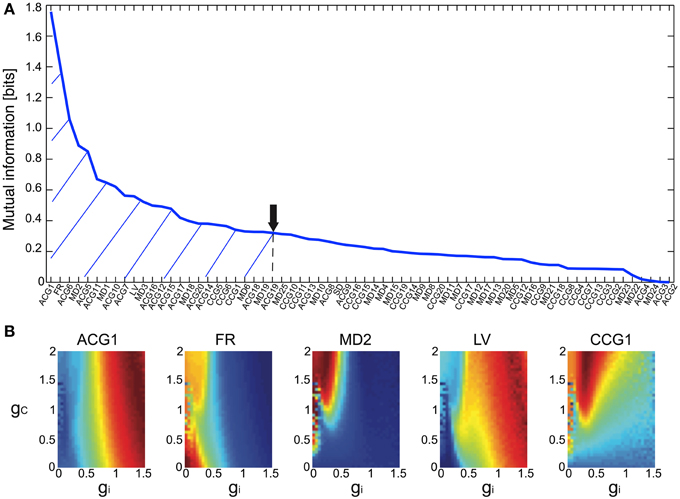
Figure 2. Mutual information of the 68 FVs and maps of five major features for g_i and g_c. (A) Mutual information concerning g_i and g_c values plotted in bits for the 68 FVs. Hatch and downward arrow indicate the 25 FVs selected for PCA. (B) 3D maps of the five representative FVs (ACG1, FR, MD2, LV, CCG1) plotting the mean of FVs for g_i and g_c by pseudo-color representation. The color-map is normalized to the peak values.

TABLE 1

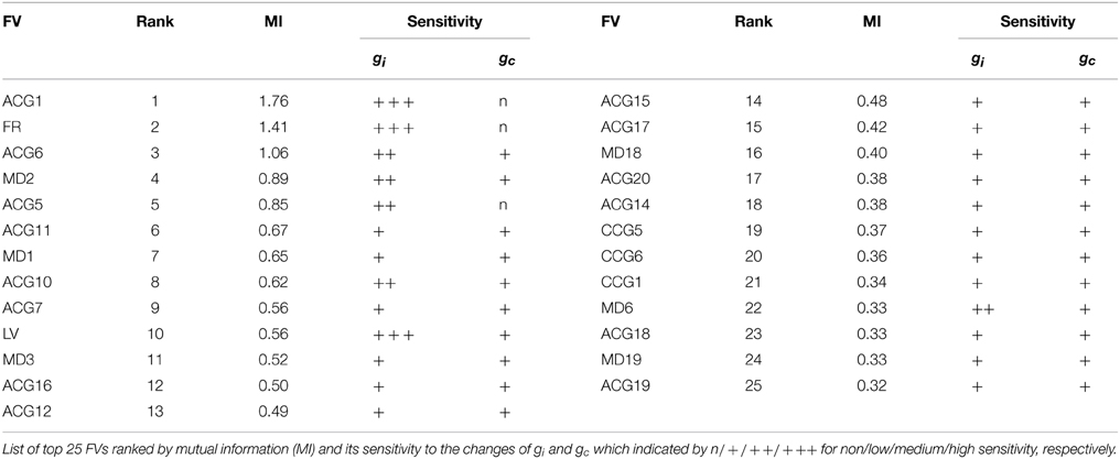
Table 1. Sensitivity of top ranked 25 FVs to changes of g_i and g_c.

We selected top three PCA axes to construct the forward models for the following two reasons. First, eigenvalues were high for the first two axes (0.27 and 0.21, respectively) and sharply decreased for the third one (0.09), with the sum of eigenvalues for the top three axes amounting up to 0.57. Second, MI was accordingly high for the first two axes (1.6 and 1.1 bits, respectively), significantly reduced for the next axis (0.63) and remained rather low for the remaining axes. These findings indicate that the top three PCA axes conveyed reliable information on the g_i and g_c.

We also studied the effects of number of FVs for three-dimensional PCA space as the evidence for Bayesian estimation (8.06E-5 for 15 FVs, 1.05E-4 for 25 FVs, and 4.88E-5 for 35 FVs), and selected the 25 FVs that exhibited the highest evidence value. They included ACG1, FR, etc., rejecting ACG2, ACG3, SD, etc. (MI and rating, 0.0001 and 68^th, 0.0017 and 67^th, and 0.25 and 32^nd, respectively). ACG1 conveyed rather high MI because it hit the first peak of ACG, but ACG2, ACG3 conveyed lower MI since they were off-focused from that peak. Those FVs were found to convey more than 70% (hatched area in Figure 2A) of the g_i and g_c information (downward arrow in Figure 2A).

3.3. Goodness of Fit of the Forward Model

PCA was conducted for a total of 1100 spike segments (10 segments each for the 110 IO neurons), containing 440 segments for 44 neurons sampled in five PIX experiments, 110 segments for 11 IO neurons sampled in two CBX experiments and 550 segments for 55 IO neurons sampled in seven CON experiments. Bayesian inference requires for the forward model of SIM data to completely cover the distribution of EXP data in the PCA space. Figures 3A–C show that this requirement is satisfied by mapping SIM (blue symbols) and EXP spike data for PIX, CBX, and CON (red, green, and black symbols) into the 3D-PCA space. We confirmed that SIM spike data completely cover the distributions of EXP spike data except for a fraction of PIX data of one animal (red diamonds).

FIGURE 3

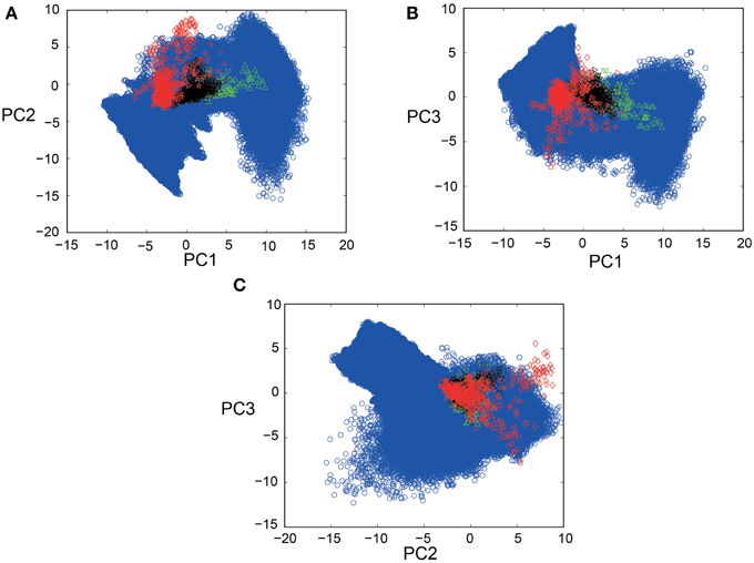
Figure 3. Scatter plots of EXP and SIM spike data in 3D-PCA space. (A–C) 2D projection views (PC1-PC2; PC1-PC3; PC2-PC3) of the scatter plots for 440, 550, and 110 spike segments for five, seven, and two animals for the PIX (red), CON (black), CBX (green) conditions, and over fifteen-million spike segments for SIM spike data (blue symbols) for 1271 combinations of g_i ([0–1.5 mS/cm²]) and g_c ([0–2.0 mS/cm²]). Note that the distribution of the SIM spike data perfectly covers that of the EXP data except for a fraction of the EXP data for one animal (red diamonds). The color conventions that represent the PIX, CON, and CBX conditions are the same in this and the following figures.

We finally constructed the forward models as mixed Gaussians fitted to the SIM spike data mapped in the PCA space and evaluated the fitting as the 3-dimensional minimum energy test of the model prediction and the SIM spike data. In general, the match was acceptable (Figure 4A), with the statistical difference being not significant (p > 0.1) for most combinations of g_i and g_c, except for few ones (about 2%) where the statistical significance was rather high (p < 0.03) (Figure 4B).

FIGURE 4

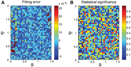
Figure 4. Goodness of fit of the forward model to the SIM spike data. (A) 3D pseudo-color representation of the fitting error of the forward model estimated as the energy test statistics between the predictions of the forward model and the SIM data plotted for g_i and g_c. (B) statistical significance of the error.

3.4. Bayesian Inference with a Relaxed Neuronal Constraint

We found that the EXP spike data were significantly non-stationary (cf. Figures 8B–D), which may cause errors in the Bayesian estimation of g_i and g_c. Those errors were minimized by the segmental Bayes whereby the entire spike data for each IO neuron was fractionated into 10 segments, Bayesian estimation of g_i and g_c was conducted segment by segment, under the commonality constraint that the g_i estimates agree between CBX and CON, and the g_c estimates between PIX and CON, respectively, and the segmental estimates were finally merged into a single estimate for every neuron (cf. Methods, Section 2.2.6) under the neuronal constraint assuming a single g_i and g_c for each neuron.

Figures 5A–D are pseudo-color representation of the posterior probability of g_i and g_c estimated for a representative IO neuron by the Bayesian inference under the commonality and the relaxed neuronal constraint (σ = 10, cf. Equation 15). The estimates were diffused broadly for all of the three conditions probably because of the fluctuations of the segmental estimates. The probability of the g_i and g_c estimates for the IO neuron for the three experimental conditions showed broad and overlapping distributions (Figures 5E,F).

FIGURE 5

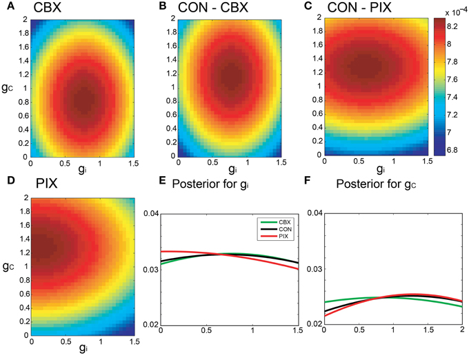
Figure 5. Segmental Bayesian estimates of g_i and g_c with relaxed commonality constraints. (A–D) Posterior probability of the g_i and g_c estimates for representative IO neurons under the relaxed commonality constraint (σ = 10) for the two experimental (CBX and PIX) and two corresponding control conditions (CON-CBX and CON-PIX). (E,F) The profiles of g_i and g_c probability of the neurons plotted in (A–D).

3.5. Bayesian Inference with a Neuronal Constraint

By contrast, the g_i and g_c of the same IO neuron as in Figure 5 estimated by Bayesian inference under the optimized neuronal constraint (σ was optimized in the range of [0.1–0.5]) were sharper, with the peak of (g_i, g_c) at (0.75, 0.75 mS/cm²) for CBX, at (0.1, 1.3 mS/cm²) for PIX and at (0.75, 1.25 mS/cm²) and (0.6, 1.3 mS/cm²) for CON-CBX and CON-PIX, respectively (Figures 6A–F). Figures 7A,B show the ensemble distributions of g_i and g_c estimated by the segmental Bayesian inference for the entire population of IO neurons in comparison with those by the non-segmental Bayes whereby g_i and g_c were estimated at once across the entire length of spike data (Figures 7C,D). The g_i and g_c estimates by the segmental Bayes essentially agreed with those by the non-segmental Bayes with the tendency for the segmental Bayesian inference to give a sharper distribution than the non-segmental Bayes. The g_i value peaked at 0.6–0.7 mS/cm² for CBX and CON and at 0.1–0.2 mS/cm² for PIX (Figures 7A,C) and the g_c for PIX and CON was 1.3 mS/cm². The g_c value for CBX was distributed diffusely across a wide range. We noted that the segmental Bayes gave rather conflicting estimates of g_c between the two animals. In one animal there was a marked leftward shift of the peak between the CBX and CON conditions (with a reduction of g_c, filled area in Figure 7B) and conversely a significant rightward shift in the other animal (open area). The non-segmental Bayesian inference also showed the same results, although the difference was less clear. The same tendency was also found in our previous study (cf. Figure 7 in Onizuka et al., 2013). Therefore this may represent reality rather than Bayesian artifacts.

FIGURE 6

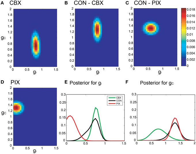
Figure 6. Segmental Bayesian estimates of g_i and g_c with optimized commonality constraints. (A–F) Similar posterior probability plots of g_i and g_c to those in Figure 5 but with the optimized commonality constraints.

FIGURE 7

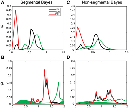
Figure 7. Segmental and non-segmental Bayes estimates for the entire IO neuronal population. (A,B) the average g_i and g_c estimates by the segmental Bayesian inference for the entire IO neuronal population. (C,D) those similar to (A,B) but by non-segmental Bayesian inference where the posterior probability was estimated across the entire spike train of the individual IO neurons. Filled and open areas in green in (B,D) represent the estimates for the two different animals in the CBX condition.

We hypothesize that the segmental Bayes minimizes the errors of g_i and g_c estimation because of the failure for the forward model to reproduce the non-stationary dynamics of IO firing. This hypothesis was tested by comparing the performance of the segmental and non-segmental Bayes in terms of the PCA error rate (the difference in the PCA scores between the EXP and the corresponding SIM spikes that were generated by the g_i and g_c estimated for those EXP spikes). PCA errors for the segmental Bayes were smaller than the non-segmental Bayes across the three experimental conditions (F = 14.18, p = 0.0002), the difference being most significant for PIX, less for CON, and insignificant for CBX (cf. solid and hatched columns Figure 8A). Correspondingly, the non-stationarity of the EXP spikes estimated as the KS distance between the distribution of the inter-spike intervals for the EXP spikes and that of Poisson and the standard deviations of the firing rate ranked in the same order as that for the significance of the PCA error difference between the segmental and non-segmental Bayes, being high, medium and low for the PIX, CON, and CBX conditions (cf. Figures 8A,C,D), respectively. These findings are consistent with our view that the segmental Bayes minimizes errors in g_i and g_c estimates because of the non-stationary dynamics of IO firing. It is notable that the corresponding SIM spikes rather faithfully reproduced the non-stationarity of the EXP spikes for the two measures across the three experimental conditions, while they were significantly smaller for the LV (Figure 8B). This finding indicates that the present simulation failed to precisely reproduce the non-stationarity estimated by the LV.

FIGURE 8

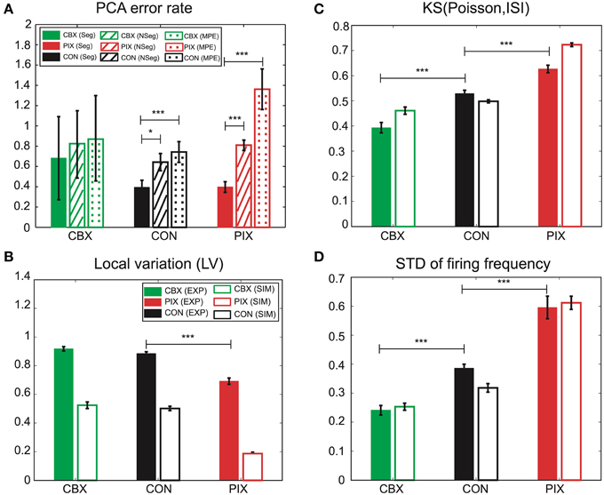
Figure 8. Performance of the segmental and non-segmental Bayesian inference and the minimum PCA error method and the non-stationarity of EXP and SIM spike data. (A) PCA error rates of the g_i and g_c estimates for the segmental (solid columns, Seg) and non-segmental (hatched, NSeg) Bayesian inference and the minimum PCA error method (dotted, MPE) averaged for the entire IO neurons for CBX, CON, and PIX conditions. The colors represent the three experimental conditions and the texture patterns represent the errors for the three methods of g_i and g_c estimates. (B–D) Non-stationality of the spike data estimated as the three metrics. (B): LV; (C): KS distance of the ISI distribution for the EXP (solid columns) and SIM (blank) spike data from Poisson distribution; (D) standard deviation of the instantaneous firing rate. The colors represent the three experimental conditions and the texture patterns represent EXP and SIM data. *p < 0.05, ***p < 0.001.

Finally, we confirmed the superiority of the segmental Bayesian inference over the minimum error method used in our previous study (Onizuka et al., 2013) in terms of the PCA error rate. The magnitude of the error rate was smaller for the segmental Bayesian inference (solid columns in Figure 8A) than that for our previous study (dotted columns) across the three experimental conditions (statistical significance, F = 23.37, p < 0.0001 by ANOVA), and the statistical significance of the error rate was largest (p < 0.0001 by t-test), moderate (p < 0.01) and minimum (p > 0.7) for the PIX, CON, and CBX conditions, respectively, corresponding to the degree of the non-stationarity of the EXP spikes. It is notable that the average number of mixed Gaussians per (g_i, g_c) grid of the forward models was three orders of magnitude smaller in the segmental Bayes (n = 8.55) than that in our previous study (n = 12,600) and slightly larger than that for the non-segmental Bayesian inference (n = 2.3), indicating that there was over- and under-fitting in the previous study and the non-segmental Bayesian inference, respectively, compared with the segmental Bayesian inference used in the present study.

4. Discussion

The goal of the present study was to resolve the inverse problem estimating the two important parameters of the IO network (i.e., g_i and g_c) by fitting the firing dynamics of the model network with those of the IO network. The parameter estimation was confronted with a huge mismatch of the model network with the brain network in the system complexity such as the granularity, the hierarchy, the degrees of freedom and the non-stationary dynamics. Consequently, the inverse problem becomes severely ill-posed (Prinz et al., 2004; Achard and Schutter, 2006), and necessitates some stochastic approaches that find the most likely solution among many possible ones according to various error functions (Geit et al., 2008).

The previous study (Onizuka et al., 2013) defined the error function as the distance between the experimental and corresponding simulation spike data in the PCA space (PCA error), constructed of various feature vectors (FVs) that are derivatives of the ISIs of the experimental spike data such as the firing rate, the auto- and cross correlation, the minimum distance (MD), the spike distance (SD), and the local variance (LV), representing the spatiotemporal firing dynamics and contained strong redundancy. In that study, the FVs were determined for short spike segments (50s) to compensate for the non-stationarity of the experimental spike trains (Grun et al., 2002; Quiroga-Lombard et al., 2013), PCA was conducted to remove the redundancy, and the g_i and g_c were determined as the ones giving the minimum PCA errors to the experimental spike segments. The minimum error method can be regarded as the extreme case of Bayesian inference where the forward model translating the model parameters into the spike features was constructed for each spike segment. This approach is equivalent to assuming different Gaussians (i.e., parameter-spike feature translation mechanisms) for every spike segment of the same single neuron and may be regarded as over-fitting.

The present study maintained the segmental approach and corrected the over-fitting by the hierarchical Bayesian inference that estimated the g_i and g_c by fitting Gaussians to every spike segment and merged them into single g_i and g_c estimates according to the neuronal constraint that assumes the same g_i and g_c for a single neuron (Figures 5, 6). This view is supported by the fact that the number of Gaussians used for construction of the forward model is three orders of magnitude smaller for the present segmental Bayesian inference than that for the minimum error method.

There were additional improvements in construction of the firing feature space in two ways. First, the FVs were selected according to the mutual information of the g_i and g_c (Figure 2) and the number of FVs (n = 25) were optimized according to the evidence function. Second, the length of the simulation spike data was expanded 10 times more than that for the previous study (from 500 to 5000 s) to ensure more satisfactory reproduction of the IO firing dynamics (Figures 3, 4). The overall performance of the segmental Bayesian inference estimated as the PCA error that is the distance between the experimental and corresponding simulation spike segments in the PCA space was generally higher across the three experimental conditions than those for the minimum PCA error method and the non-segmental Bayesian inference that estimated the g_i and g_c across the entire spike length (Figure 8A). The statistical significance of the difference was high, modest and minimal in the PIX, CON, and CBX conditions, respectively, in correspondence with the non-stationarity of the IO firing evaluated as the three metrics, including the KS distance of the ISIs from Poisson distributions, the LV, and the standard deviation of the firing rate (Figures 8B–D). The segmental Bayes could be regarded as a way to minimize estimation errors of g_i and g_c due to the errors of the current forward model to precisely reproduce the non-stationality of IO firing. Allowance of fluctuations for segmental g_i and g_c estimates is equivalent to recent methods (Arridge et al., 2006; Huttunen and Kaipio, 2007; Kaipio and Somersalo, 2007) to reduce parameter estimation errors due to modeling errors by assuming system noise.

These findings indicate that segmental Bayesian inference performs better than the other two methods in cases of highly non-stationary firing dynamics. The estimates of g_i and g_c by the segmental Bayesian inference are in partial agreement with those of our previous study. The point of agreement was the g_c for the CON and PIX conditions (1.21±0.2 and 1.16±0.43 mS/cm² for the present and previous studies) and those of disagreement were g_c for the CBX condition (1.24±0.6 and 0.75±0.51 mS/cm²) and g_i for the CON (0.54±0.18, 1.10±0.36 mS/cm²), PIX (0.1±0.04, 0.51±0.41 mS/cm²), and CBX conditions (0.65±0.15, 1.11±0.34 mS/cm²). The present estimates may be more accurate than the previous ones for the three reasons. First, we expanded the g_c range for simulation (from [0–1.6 mS/cm²] in the previous study to [0–2.0 mS/cm²] in the present study), second, we expanded the data length for simulation (from 500 to 5000 s) for better simulation of experimental spike dynamics, and third, the present estimates gave smaller PCA errors (0.39±0.05, 0.68±0.41, 0.39±0.07 under PIX, CBX and CON in present study and 1.36±0.20, 0.86±0.42, 0.74±0.10 in our previous study).

The g_c estimates for the CBX condition diverged between two animals in the present study (Figure 7B), and the same tendency was also found in our previous study, although this tendency was less clear. The reason for this discrepancy between the two animals is unclear. CBX is a nonspecific blocker of the gap-junctional conductance and may act on other ionic conductances than the gap-junction, affecting the g_c estimates. The IO units were sampled across many micro-zones of the cerebellum on which the gap-junctional conductance was dependent, being high and low in the same and different micro-zones, respectively. This heterogeneity in the g_c population may also be the cause of the discrepancy.

Conflict of Interest Statement

The authors declare that the research was conducted in the absence of any commercial or financial relationships that could be construed as a potential conflict of interest.

Acknowledgments

This research was conducted under the support by the National Institute of Information and Communications Technology. HH, OY, MS, MK, and KT was supported by a contract with the National Institute of Information and Communications Technology entitled ‘Development of network dynamics modeling methods for human brain data simulation systems’. HH was supported by Grants-in-Aid for Scientific Research for the Japan Society for the Promotion of Science (JSPS) Fellows. IT was supported by Grants-in-Aid for Scientific Research (No. 25293053) from MEXT of Japan.

References

Achard, P., and Schutter, E. D. (2006). Complex parameter landscape for a complex neuron. PLoS Comput. Biol., 2:e94. doi: 10.1371/journal.pcbi.0020094

PubMed Abstract | CrossRef Full Text | Google Scholar

Arridge, S., Kaipio, J. S., Kolehmainen, V., Schweiger, M., Somersalo, E., Tarvainen, T., et al. (2006). Approximation errors and model reduction with an application in optical diffusion tomography. Inverse Probl. 22, 175–196. doi: 10.1088/0266-5611/22/1/010

CrossRef Full Text | Google Scholar

Aslan, B., and Zech, G. (2005). Statistical energy as a tool for binning-free, multivariate goodness-of-fit tests, two-sample comparison and unfolding. Nucl. Instrum. Methods Phys. Res. A 537, 626–636. doi: 10.1016/j.nima.2004.08.071

CrossRef Full Text | Google Scholar

Berg, R. W., and Ditlevsen, S. (2013). Synaptic inhibition and excitation estimated via the time constant of membrane potential fluctuations. J. Neurophysiol. 110, 1021–1034. doi: 10.1152/jn.00006.2013

PubMed Abstract | CrossRef Full Text | Google Scholar

Best, A. R., and Regehr, W. G. (2009). Inhibitory regulation of electrically coupled neurons in the inferior olive is mediated by asynchronous release of gaba. Neuron 62, 555–565. doi: 10.1016/j.neuron.2009.04.018

PubMed Abstract | CrossRef Full Text | Google Scholar

Bishop, C. M. (2006). Pattern Recognition and Machine Learning. New York, NY: Springer.

Google Scholar

Blenkinsop, T. A., and Lang, E. J. (2006). Block of inferior olive gap junctional coupling decreases purkinje cell complex spike synchrony and rhythmicity. J. Neurosci. 26, 1739–1748. doi: 10.1523/JNEUROSCI.3677-05.2006

PubMed Abstract | CrossRef Full Text | Google Scholar

Fairhurst, D., Tyukin, I., Nijmeijer, H., and Leeuwen, C. V. (2010). Observers for canonic models of neural oscillators. Math. Model. Nat. Phenom. 5, 146–184. doi: 10.1051/mmnp/20105206

PubMed Abstract | CrossRef Full Text | Google Scholar

Geit, W. V., Schutter, E. D., and Achard, P. (2008). Automated neuron model optimization techniques: a review. Biol. Cybern. 99, 241–251. doi: 10.1007/s00422-008-0257-6

PubMed Abstract | CrossRef Full Text | Google Scholar

Gelman, A., Carlin, J., Stern, H., Dunson, D., Vehtari, A., and Rubin, D. B. (2013). Bayesian Data Analysis, 3rd Edn. Boca Raton, FL: CRC Press; Taylor & Francis Group.

Google Scholar

Grun, S., Diesmann, M., and Aertsen, A. (2002). Unitary events in multiple single-neuron spiking activity. ii. nonstationary data. Neural Compt. 14, 81–119. doi: 10.1162/089976602753284464

PubMed Abstract | CrossRef Full Text | Google Scholar

Hirata, Y., and Aihara, K. (2009). Representing spike trains using constant sampling intervals. J. Neurosci. Methods 183, 277–286. doi: 10.1016/j.jneumeth.2009.06.030

PubMed Abstract | CrossRef Full Text | Google Scholar

Hoge, G., Davidson, K., Yasumura, T., Castillo, P., Rash, J., and Pereda, A. (2011). The extent and strength of electrical coupling between inferior olivary neurons is heterogeneous. J. Neurophysiol. 105, 1089–1101. doi: 10.1152/jn.00789.2010

PubMed Abstract | CrossRef Full Text | Google Scholar

Huttunen, J., and Kaipio, J. (2007). Approximation errors in nonstationary inverse problems. Inverse Probl. Imag. 1, 77–93. doi: 10.3934/ipi.2007.1.77

CrossRef Full Text | Google Scholar

Ikeda, K., Otsuka, K., and Matsumoto, K. (1989). Maxwell-bloch turbulence. Prog. Theor. Phys. Suppl. 99, 295–324. doi: 10.1143/PTPS.99.295

CrossRef Full Text | Google Scholar

Kaipio, J., and Somersalo, E. (2007). Statistical inverse problems: discretization, model reduction and inverse crimes. J. Comp. Appl. Math. 198, 493–504. doi: 10.1016/j.cam.2005.09.027

CrossRef Full Text | Google Scholar

Kaneko, K. (1990). Clustering, coding, switching, hierarchical ordering, and control in a network of chaotic elements. Physica D 41, 137–172. doi: 10.1016/0167-2789(90)90119-A

CrossRef Full Text | Google Scholar

Keren, N., Peled, N., and Korngreen, A. (2005). Constraining compartmental models using multiple voltage recordings and genetic algorithms. J. Neurophysiol. 94, 3730–3742. doi: 10.1152/jn.00408.2005

PubMed Abstract | CrossRef Full Text | Google Scholar

Kirkpatrick, S., Gelatt, C. D. Jr., and Vecchi, M. P. (1983). Optimization by simulated annealing. Science 220, 671–680. doi: 10.1126/science.220.4598.671

PubMed Abstract | CrossRef Full Text | Google Scholar

Kitazono, J., Omori, T., Aonishi, T., and Okada, M. (2012). Estimating membrane resistance over dendrite using markov random field. IPSJ Trans. Mathe. Model. Appl. 5, 89–94. doi: 10.2197/ipsjtrans.5.186

CrossRef Full Text | Google Scholar

Kreuz, T., Chicharro, D., Houghton, C., Andrzejak, R., and Mormann, F. (2013). Monitoring spike train synchrony. J. Neurophysiol. 109, 1457–1472. doi: 10.1152/jn.00873.2012

PubMed Abstract | CrossRef Full Text | Google Scholar

Lang, E. J. (2002). GABAergic and glutamatergic modulation of spontaneous and motor-cortex-evoked complex spike activity. J. Neurophysiol. 87, 1993–2008. doi: 10.1152/jn.00477.2001

PubMed Abstract | CrossRef Full Text | Google Scholar

Lang, E. J., Sugihara, I., and Llinas, R. (1996). Gabaergic modulation of complex spike activity by the cerebellar nucleoolivary pathway in rat. J. Neurophysiol. 76, 255–275.

PubMed Abstract | Google Scholar

Llinas, R., Baker, R., and Sotelo, C. (1974). Electrotonic coupling between neurons in cat inferior olive. J. Neurophysiol. 37, 560–571.

PubMed Abstract | Google Scholar

Llinas, R., and Yarom, Y. (1981). Electrophysiology of mammalian inferior olivary neurones in vitro. different types of voltage-depedent ionic conductances. J. Physiol. 315, 549–567. doi: 10.1113/jphysiol.1981.sp013763

PubMed Abstract | CrossRef Full Text | Google Scholar

Manor, Y., Rinzel, J., Segev, I., and Yarom, Y. (1997). Low-amplitude oscillations in the inferior olive: a model based on electrical coupling of neurons with heterogeneous channel densities. J. Neurophysiol. 77, 2736–2752.

PubMed Abstract | Google Scholar

Meng, L., Kramer, M. A., and Eden, U. T. (2011). A sequential monte carlo approach to estimate biophysical neural models from spikes. J. Neural Eng. 8, 065006. doi: 10.1088/1741-2560/8/6/065006

PubMed Abstract | CrossRef Full Text | Google Scholar

Nikolenko, V., Poskanzer, K. E., and Yuste, R. (2007). Two-photon photostimulation and imaging of neural circuits. Nat. Methods 4, 943–950. doi: 10.1038/nmeth1105

PubMed Abstract | CrossRef Full Text | Google Scholar

Onizuka, M., Hoang, H., Kawato, M., Tokuda, I. T., Schweighofer, N., Katori, Y., et al. (2013). Solution to the inverse problem of estimating gap-junctional and inhibitory conductance in inferior olive neurons from spike trains by network model simulation. Neural Netw 47, 51–63. doi: 10.1016/j.neunet.2013.01.006

PubMed Abstract | CrossRef Full Text | Google Scholar

Pastrana, E. (2010). Optogenetics: controlling cell function with light. Nat. Methods 8, 24–25. doi: 10.1038/nmeth.f.323

CrossRef Full Text | Google Scholar

Prinz, A. A., Bucher, D., and Marder, E. (2004). Similar network activity from disparate circuit parameters. Nat. Neurosci. 7, 1345–1352. doi: 10.1038/nn1352

PubMed Abstract | CrossRef Full Text | Google Scholar

Quiroga-Lombard, C. S., Hass, J., and Durstewitz, D. (2013). Method for stationary segmentation of spike train data with application to the pearson cross-correlation. J. Neurophysiol. 110, 562–572. doi: 10.1152/jn.00186.2013

PubMed Abstract | CrossRef Full Text | Google Scholar

Sato, M. (2001). On-line model selection based on the variational bayes. Neural Compt. 13, 1649–1681. doi: 10.1162/089976601750265045

CrossRef Full Text | Google Scholar

Schweighofer, N., Doya, K., Chiron, J. V., Fukai, H., Furukawa, T., and Kawato, M. (2004). Chaos may enhance information transmission in the inferior olive. Proc. Natl. Acad. Sci.U.S.A. 101, 4655–4660. doi: 10.1073/pnas.0305966101

PubMed Abstract | CrossRef Full Text | Google Scholar

Shinomoto, S., Miura, K., and Koyama, S. (2005). A measure of local variation of inter-spike intervals. Biosystems 79, 67–72. doi: 10.1016/j.biosystems.2004.09.023

PubMed Abstract | CrossRef Full Text | Google Scholar

Torben-Nielsen, B., Segev, I., and Yarom, Y. (2012). The generation of phase differences and frequency changes in a network model of inferior olive subthreshold oscillations. PLoS Comput. Biol. 8:e1002580. doi: 10.1371/journal.pcbi.1002580

PubMed Abstract | CrossRef Full Text | Google Scholar

Tsuda, I. (1992). Dynamics link of memory - chaotic memory map in nonequilibirum neural networks. Neural Netw. 5, 313–326. doi: 10.1016/S0893-6080(05)80029-2

CrossRef Full Text | Google Scholar

Tsuda, I., Fujii, H., Todokoro, S., Yasuoka, T., and Yamaguchi, Y. (2004). Chaotic itinerancy as a mechanism of irregular changes between synchronization and desynchronization in a neural network. J. Integr. Neurosci. 3, 159–182. doi: 10.1142/S021963520400049X

PubMed Abstract | CrossRef Full Text | Google Scholar

Tsunoda, T., Omori, T., Miyakawa, H., Okada, M., and Aonishi, T. (2010). Estimation of intracellular calcium ion concentration by nonlinear state space modeling and expectation maximization algorithm for parameter estimation. J. Phys. Soc. Jpn 79:124801. doi: 10.1143/JPSJ.79.124801

CrossRef Full Text | Google Scholar

Tyukin, I., Steur, E., Nijmeijer, H., Fairhurst, D., Song, I., Semyanov, A., et al. (2010). State and parameter estimation for canonic models of neural oscillators. Int. J. Neural Syst. 20, 193–207. doi: 10.1142/S0129065710002358

PubMed Abstract | CrossRef Full Text | Google Scholar

Vanier, M. C., and Bower, J. M. (1999). A comparative survey of automated parameter search methods for compartmental neural models. J. Comput. Neurosci. 7, 149–171. doi: 10.1023/A:1008972005316

PubMed Abstract | CrossRef Full Text | Google Scholar