Extended Model-Based Feedforward Compensation in ℒ1 Adaptive Control for Mechanical Manipulators: Design and Experiments

1. Introduction

Adaptive control of mechanical manipulators has gained an increased interest in the last few decades. Indeed, for an efficient control of such systems, uncertainties, external disturbances, and variations in the dynamics have to be considered in the control scheme design. Since conventional non-adaptive model-based controllers rely mainly on the dynamic model of the manipulator, they may fail if this last one is not sufficiently accurate. This is the case when some phenomena are not modeled (e.g., friction, actuators’ dynamics, etc.) or when simplifying hypotheses are considered without careful analysis. In both cases, the controller will not be able to keep the desired performance and may even lead to instability of the closed-loop system. In such situation, adaptive control seems to be the appropriate solution to overcome these shortcomings. Indeed, adaptive controllers are mainly known for their ability to estimate unknown, varying, or uncertain parameters of the system and its environment and to adapt the controller accordingly.

The earlier designed adaptive controllers were mainly based on model reference adaptive control (MRAC). These controllers hold the advantage of not relying on any knowledge of the dynamics of the system. MARC-based strategies were mainly applied on serial manipulators. For instance, a decentralized control scheme based on MRAC has been proposed in Dubowsky and DesForges (1979) to control a 3-DOFs robotic arm. In this work, the manipulator was supposed to be controlled by a PD feedback loop with adjustable gains. The step response of each joint of the manipulator had to follow a user-defined step response generated by a second order reference model. However, a very restrictive assumption was made in this study that the coupling between the different joints was neglected. A more sophisticated controller based on MRAC was proposed in Horowitz and Tomizuka (1986), where the coupled dynamics of the manipulator has been explicitly considered in the controller design. In this work, the proposed control law consists of a fixed PD feedback loop in addition to an adaptive loop intended to compensate for non-linearities of the system. However, this controller was not suitable for real-time setups. In fact, the number of the controller parameters to be estimated was too large (11 parameters for a simple 3-DOFs manipulator, after simplification). In addition to these issues, MRAC inherently suffers from a major drawback; the estimation and the control loops are coupled (Hovakimyan and Cao, 2010). This is mainly due to the fact that the adaptive gain in MRAC acts as a feedback gain, meaning that a trade-off has to be made between the speed of adaptation and the robustness of the controller. Recently, a new strategy called ℒ₁ adaptive control has been developed in order to overcome this problem (Cao and Hovakimyan, 2006a,b). The ℒ₁ adaptive control structure features a unique filtering technique that enables a decoupling between the estimation and the control loops. This means that the adaptation can be made arbitrarily fast while guaranteeing sufficient robustness margins.

With the advances in modeling techniques, obtaining an accurate dynamic model for a robot manipulator became relatively an easy task (Merlet, 2006). Consequently, model-based controllers that take advantage of the dynamics knowledge in the control design captured an increasing attention. Craig et al. proposed in Craig et al. (1987) an adaptive version of the computed-torque control scheme (Markiewicz, 1973). However, the proposed controller showed several limitations that restricted its real-time implementation (e.g., joint accelerations had to be measured). Later on, several improvements have been brought to model-based adaptive control resulting in more reliable, simpler, and more efficient adaptive schemes (Slotine and Weiping, 1987; Ortega and Spong, 1989; Sadegh and Horowitz, 1990; Shang and Cong, 2010). One particular control strategy that caught our attention is the desired compensation adaptation law (DCAL) proposed in Sadegh and Horowitz (1990). DCAL features many advantageous characteristics that make it suitable for real-time implementation. One interesting feature, among others, is that it relies on the desired trajectories of the manipulator instead of the measured ones, which means that it is less sensitive to measurement noise and enables offline computation of some terms in the control law. Nevertheless, one common drawback of model-based controllers is that the non-modeled dynamics are not taken into consideration by the adaptive loop. Instead, the feedback loop (usually a PD) is in charge of rejecting the eventual residual non-linearities. Though a PD feedback loop is usually sufficient for slow accelerations, the performance on high speeds may be improved by using more sophisticated feedback actions (Bennehar et al., 2014a,b).

In this paper, a new adaptive control scheme is proposed, it combines the benefits of both ℒ₁ and model-based adaptive control. It was shown in (Bennehar et al., 2015) that ℒ₁ adaptive control applied to a 4-DOFs PKM outperforms the PD controller in terms of tracking performance. In this work, we further improve ℒ₁ adaptive control by augmenting it with a model-based adaptive term that accounts for the modeling uncertainties with known structure. We compare the performance of both ℒ₁ adaptive controller and the augmented one through real-time experiments on a new 4-DOFs RA-PKM developed in our laboratory. The remainder of this paper is organized as follows. In section 2, the dynamic modeling, required for the proposed controller design, is addressed. In section 3, a background on ℒ₁ adaptive control for mechanical manipulators is provided. The main contribution of the actual paper, being a new controller based on ℒ₁ and model-based adaptive control and its application to RA-PKMs are detailed in section 4. Real-time experiments performed on ARROW and the obtained results are presented and discussed in section 5. Finally, conclusions are drawn in section 6.

2. Dynamic Modeling of the Plant: The Arrow Robot

ARROW (acronym for Accurate and Rapid Robot with large Operational Workspace) is a 4-DOF RA-PKM intended to be used for fast lightweight machining tasks. It has two degrees of actuation redundancy since it is equipped with six linear actuators and has four degrees of freedom. All the actuators are aligned along the same axis and are split into two sets, each set consists of three actuators (cf. Figure 1). The actuators are connected to the end affecter through two pairs of simple arms and one pair of parallelograms. As its acronym indicates, the ARROW robot, developed in the framework of the French ANR-ARROW project, has been designed in the aim of creating a very fast and accurate PKM with large workspace and homogeneous performance throughout its workspace. Moreover, its platform is capable of performing ±90° rotations free of any singularities. The CAD design of ARROW is shown in Figure 1 and its main geometrical and dynamical parameters are summarized in Table 1. A more detailed description about the design theory and the development of ARROW robot can be found in Shayya (2015).

FIGURE 1

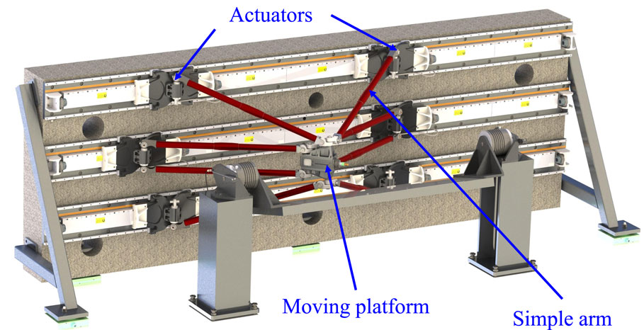
Figure 1. CAD schematic view of ARROW PKM.

TABLE 1

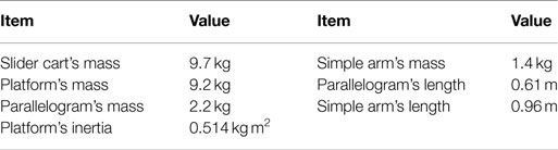
Table 1. Main parameters of ARROW PKM.

For the subsequent control development, the establishment of the dynamic model of ARROW is required. The latter will be included in the control scheme design in order to enhance the dynamic performance and tracking capabilities of the robot. First, let us enumerate the considered hypotheses, mainly common to PKMs (Corbel et al., 2010), in order to simplify the establishment of the dynamic model:

1. Both dry and viscous friction forces are neglected since all active and passive joints are designed such as to minimize friction effects, even though, their insignificant effect could be considered in control as it will be explained later on.

2. The mass of each arm is split up into two halves being located at the end tips of the arm. Hence, the influence of the mass of the arms is considered with the actuators and the platform. This assumption can be justified by the small mass of the arms compared to the other components. Similarly, the mass of the parallelograms is also split up into two halves and considered in both the dynamics of the actuators and the moving platform.

Applying the law of motion, the dynamics of the actuators are given by the following equation (Shayya et al., 2014):

$M_a\ddot{q}=\mathrm{\Gamma }-J_q^{T}f$ (1)

being M_a = diag(m_as, m_as, m_ap, m_ap, m_as, m_as), where m_as includes the mass of the actuator, the moving cart, and the half-mass of the simple arm. m_ap includes the mass of the actuator, the moving cart, and the half-mass of the parallelogram (i.e., two simple arms). $\ddot{q}$ ∈ ℝ⁶ is the joint acceleration vector, Γ ∈ ℝ⁶ is the input force vector, J_q ∈ ℝ^6×6 is the joint Jacobian matrix, and f ∈ ℝ⁶ is the force vector resulting from acceleration and gravitational forces acting on the moving platform. From the platform side, the dynamics are governed by Shayya et al. (2014)

$M_p\ddot{X}+{\Lambda }_c\dot{X}=J_x^{T}f+m_{p}G$ (2)

where M_p ∈ ℝ^4×4 is the inertia matrix of the moving platform, $\ddot{X}\in {ℝ}^4$ is its acceleration vector, Λ_c ∈ ℝ^4×4 is the matrix of Coriolis and centrifugal effects, $\dot{X}\in {ℝ}^4$ is the velocity vector of the moving platform, J_x ∈ ℝ^6×4 is the Cartesian Jacobian matrix, m_p is the total mass of the platform, including the half-masses from the arms and parallelograms and G = [0, 0, −10,0]^T m/s² is the gravity wrench acting on the platform. The Jacobian matrices Jq and J_x links the joint velocities and those of the moving platform according to the following relationship:

$J_q\dot{q}=J_x\dot{X}$ (3)

where $\dot{q}\in {ℝ}^6$ is the joint velocities and $\dot{X}\in {ℝ}^4$ denotes the velocities of the moving platform. Solving for f in (1) and substituting the resulting equation in (2) while replacing $\ddot{q}=J_m\ddot{X}+{\dot{J}}_m\dot{X}$, where $J_m=J_q^{-1}{J}_x$ the inverse Jacobian matrix, yields the following equation:

$\ddot{X}=H\mathrm{\Gamma }-\Lambda \dot{X}+A_G$ (4)

where H ∈ ℝ^4×6, Λ ∈ ℝ^4×4, and A_G ∈ ℝ⁴ are expressed by

$\left\{\begin{array}{cc}H={\left(M_p+J_m^T{M}_a{J}_m\right)}^{-1}{J}_m^T\hfill & \hfill \\ \Lambda =H{M}_a{\dot{J}}_m+{\left(M_p+J_m^T{M}_a{J}_m\right)}^{-1}{\Lambda }_c\hfill & \hfill \\ A_G={\left(M_p+J_m^T{M}_a{J}_m\right)}^{-1}{m}_{p}G\hfill \end{array}\right.$

Equation (4) is referred to as the simplified direct dynamic model (SDDM) of ARROW robot, which is unique. However, the inverse dynamic model (IDM), required for model-based control schemes, is not unique due to actuation redundancy. It is usually obtained by using the pseudo-inverse of the matrix H as follows

$H^{+}\left(\ddot{X}+\Lambda \dot{X}-A_G\right)=\mathrm{\Gamma }$ (5)

where H⁺ denotes the pseudo-inverse of H. The inverse dynamic model of ARROW robot, given by (5), is expressed in terms of the Cartesian coordinates of the moving platform and is suitable for Cartesian-space control. To express these dynamics in terms of joint coordinates instead of Cartesian ones, which is suitable for joint-space control, the inverse Jacobian matrix can be used to yield

$H^{+}\left(J_m^{+}\ddot{q}+\left(\Lambda J_m^{+}-J_m^{+}{J}_m{J}_m^{+}\right)\dot{q}-A_G\right)=\mathrm{\Gamma }$ (6)

where $J_m^{+}$ is the pseudoinverse of J_m. The dynamics of ARROW robot in equation (6) can be rewritten into the standard joint space form of rigid multibody manipulators as follows:

$M\left(q\right)\ddot{q}+C\left(q,\dot{q}\right)\dot{q}+G\left(q\right)=\mathrm{\Gamma }$ (7)

being the dynamic matrices M(q), $C\left(q,\dot{q}\right)$ and G(q) given by

$\left\{\begin{array}{cc}M\left(q\right)=H^{+}{J}_m^{+}\hfill & \hfill \\ C\left(q,\dot{q}\right)=H^{+}\Lambda J_m^{+}-J_m^{+}{J}_m{J}_m^{+}\hfill & \hfill \\ G\left(q\right)=-H^{+}{A}_G\hfill \end{array}\right.$

For more details about the kinematic and dynamic modeling of ARROW robot, the reader is referred to Shayya (2015).

3. Background on ℒ₁ Adaptive Control

Consider the set of desired joint trajectories q_d ∈ ℝⁿ to be tracked by the active joints (linear actuators in the case of ARROW robot) of the manipulator to be controlled. These trajectories are issued from a trajectory generator in Cartesian space according to the task to be performed. Then the corresponding joint trajectories are computed by solving the inverse kinematics problem (IK), which is trivial in the case of PKMs. For the subsequent control development and to quantify the tracking errors, consider the following position-velocity combined tracking error:

$r\left(t\right)=\left(\dot{q}\left(t\right)-{\dot{q}}_d\left(t\right)\right)+\mathrm{\lambda }\left(q\left(t\right)-q_d\left(t\right)\right)$ (8)

where λ ∈ ℝ⁺ is a control design parameter. Let us now introduce the following control input that is the combination of two distinct terms:

$\mathrm{\Gamma }\left(t\right)={\mathrm{\Gamma }}_m\left(t\right)+{\mathrm{\Gamma }}_{\mathit{AD}}\left(t\right),{\mathrm{\Gamma }}_m\left(t\right)\triangleq A_{m}r\left(t\right)$ (9)

where A_m ∈ ℝ^n×n is a user-defined Hurwitz matrix that characterizes the desired transient response of the system. In equation (9), the first term [i.e., A_mr(t)] is a stabilizing state feedback term while Γ_AD (t) is an adaptive term and will be explained later on. Substituting the control law (9) in (7) yields the following equation that governs the evolution of the combined tracking error:

$\dot{r}\left(t\right)=A_{m}r\left(t\right)+{\mathrm{\Gamma }}_{\mathit{AD}}\left(t\right)-\mathrm{\eta }\left(t,\mathrm{\zeta }\left(t\right)\right),r\left(0\right)=r_0$ (10)

where the non-linear function η(t, ζ(t)) with ζ = [r,q]^T gathers all the remaining non-linearities of the system that result from the application of the control law in (9). These non-linearities may include both known and unknown quantities such as modeling non-linearities, uncertainties, external disturbances, and so on. Under some reasonable assumptions, the non-linear function η(t, ζ(t)) can be parameterized using some parameters θ(t), σ(t) ∈ ℝⁿ and the Λ_∞ norm of the combined tracking error as follows (Hovakimyan and Cao, 2010):

$\mathrm{\eta }\left(t,\mathrm{\zeta }\left(t\right)\right)=\mathrm{\theta }\left(t\right)\parallel r_t{\parallel }_{{ℒ}_{\infty }}+\mathrm{\sigma }\left(t\right).$ (11)

Substituting equation (11) in equation (10), the combined tracking error becomes

$\dot{r}\left(t\right)=A_{m}r\left(t\right)+{\mathrm{\Gamma }}_{\mathit{AD}}\left(t\right)-\left(\mathrm{\theta }\left(t\right)\parallel r_t{\parallel }_{{ℒ}_{\infty }}+\mathrm{\sigma }\left(t\right)\right).$ (12)

In an ideal scenario, where all the non-linearities considered in η(t, ζ(t)) are perfectly known (i.e., perfect knowledge of the dynamic model, no immeasurable disturbances, no uncertainties, etc.), replacing ${\mathrm{\Gamma }}_{\mathit{AD}}\left(t\right)=\mathrm{\eta }\left(t,\mathrm{\zeta }\left(t\right)\right)=\left(\mathrm{\theta }\left(t\right)\parallel r_t{\parallel }_{{ℒ}_{\infty }}+\mathrm{\sigma }\left(t\right)\right)$ in equation (9) should compensate for all the non-linearities resulting in the desired error dynamics specified by A_m as follows:

$\dot{r}\left(t\right)=A_{m}r\left(t\right).$ (13)

However, in practical situations, the dynamics of the robot is either uncertain or unknown. Furthermore, the external disturbances acting on the system are often immeasurable, and hence, could not be accounted for by a specific control term. Consequently, the adaptive control component Γ_AD(t) should be carefully designed in order to appropriately estimate the non-linear function η(t, ζ(t)) in real-time. To that end, consider the following state predictor of the dynamics of the combined tracking error:

$\begin{array}{ll}\hfill \dot{\widehat{r}}\left(t\right)& =A_m\widehat{r}\left(t\right)+{\mathrm{\Gamma }}_{\mathit{AD}}\left(t\right)-\left(\widehat{\theta }\left(t\right)\parallel r_t{\parallel }_{{ℒ}_{\infty }}+\widehat{\sigma }\left(t\right)\right)-K\tilde{r}\left(t\right),\widehat{r}\left(0\right)=r_0\end{array}$ (14)

where $\widehat{r}\left(t\right)\in {ℝ}^n$ is the prediction of r(t), $\tilde{r}\left(t\right)\triangleq \widehat{r}\left(t\right)-r\left(t\right)$ is the prediction error, and K ∈ ℝ^n×n is a design matrix introduced to reject high frequency noises (Nguyen et al., 2013). $\widehat{\theta }\left(t\right)$ and $\widehat{\sigma }\left(t\right)$ are the estimates of θ(t) and σ(t), respectively, generated according to the following projection-based adaptation rules:

$\begin{array}{ll}\hfill \dot{\widehat{\theta }}\left(t\right)& =\Sigma \text{Proj}\left(\widehat{\theta }\left(t\right),P\tilde{r}\left(t\right)\parallel r_t\parallel {ℒ}_{\infty }\right),\widehat{\theta }\left(0\right)={\widehat{\theta }}_0\end{array}$ (15)

$\begin{array}{ll}\hfill \dot{\widehat{\sigma }}\left(t\right)& =\Sigma \text{Proj}\left(\widehat{\sigma }\left(t\right),P\tilde{r}\left(t\right)\right),\widehat{\sigma }\left(0\right)={\widehat{\sigma }}_0\end{array}$ (16)

where Σ is a positive adaptation gain and P = P^T > 0 is the solution to the algebraic Lyapunov equation $A_m^{T}P+P{A}_m=-Q$, for some arbitrary matrix Q = Q^T > 0. The projection operator Proj in equations (15) and (16) prohibits the estimated values from exceeding their allowable range specified in the control design (i.e., $\parallel \widehat{\theta }(t){\parallel }_{{}_{\infty }}<{\theta }_b,\parallel \widehat{\sigma }(t){\parallel }_{{}_{\infty }}<{\sigma }_b,\forall t>0,{\theta }_b,{\sigma }_b\in {ℝ}^{+}$). The adaptive control term in (9) is the output of

${\mathrm{\Gamma }}_{\mathit{AD}}\left(s\right)=C\left(s\right)\widehat{\eta }\left(s\right)$ (17)

where $\widehat{\eta }\left(s\right)$ is the Laplace transform of $\widehat{\eta }\left(t\right)=\left(\widehat{\theta }\left(t\right)\parallel r_t{\parallel }_{{ℒ}_{\infty }}+\widehat{\sigma }\left(t\right)\right)$ and C(s) is a diagonal matrix of BIBO-stable¹ strictly proper transfer functions with DC gain (Khalil, 2002). This particular structure, according to ℒ₁ adaptive control theory, decouples the estimation loop from the control loop that allows for arbitrarily large gains without hurting robustness.

4. Proposed Solution: An Extended L1 Adaptive Control

In order to improve the performance of ℒ₁ adaptive control, we propose to include the dynamics of the manipulator in the control scheme design. Furthermore, we want the additional dynamic-based term to be able to adapt its parameters to the possible variations in the robot and its environment (e.g., handling a payload with unknown dynamic properties, interaction with the environment, etc.). Though the dynamic parameters of the robot may be known, one should consider the scenario where these values may be varying or inaccurately known. The current section highlights the main contribution of this paper as it describes how the robot’s dynamics knowledge is included in the control law and how it is supposed to improve the control performance of the manipulator.

4.1. Linear-in-the-Parameters Formulation of the Dynamics

For model-based adaptive control schemes, a reformulation of the dynamics is required (Craig et al., 1987). The unknown or uncertain parameters to be estimated in real-time have to be separated from the non-linear functions in the dynamic model.

Consider the following dynamic model of a n-DOFs mechanical manipulator in joint space:

$M\left(q\right)\ddot{q}+C\left(q,\dot{q}\right)+G\left(q\right)=\mathrm{\Gamma }\left(t\right)$ (18)

where M(q) ∈ ℝ^n×n is the symmetric, positive definite inertia matrix, $N\left(q,\dot{q}\right)\in {ℝ}^n$ gathers Coriolis, centrifugal, and gravity forces, and Γ ∈ ℝⁿ is the input vector. M(q) and $N\left(q,\dot{q}\right)$ are usually composed of non-linear functions of the joint position and velocity vectors. These non-linear terms, however, appear in a linear form with respect to the robot’s geometric and dynamic parameters. Consequently, the dynamics in (18) can be rewritten in the following linear form:

$M\left(q\right)\ddot{q}+C\left(q,\dot{q}\right)+G\left(q\right)=Y\left(q,\dot{q},\ddot{q}\right)\mathrm{\Theta }$ (19)

where Y (.) ∈ ℝ^n×p is called the regression matrix that is a non-linear function of $q,\dot{q}$ and $\ddot{q}$, Θ ∈ ℝ^p is the vector of the parameters of the manipulator to be estimated. It is worth to note that the formulation in (19) is not unique, it actually depends on the set of chosen parameters. Besides, the estimated elements within the parameters vector can either appear in a separate form or as a combination of different parameters. Examples of the dynamics reformulation for some manipulators can be found in Craig et al. (1987) and Sadegh and Horowitz (1990).

4.2. Proposed Control Solution: Augmented ℒ₁ Adaptive Control with Adaptive Feedforward

The ℒ₁ adaptive control law described in section 3 consists into two separate terms. The first one is a stabilizing state feedback term, while the second one is the adaptive term in charge of compensating the system uncertainties to achieve the desired performance. Thus, the adaptive term in ℒ₁ adaptive control is responsible for compensating both structured (i.e., modeled) and unstructured (i.e., not included in the model such as friction) uncertainties. Nevertheless, since we have in disposal a dynamic model of our manipulator, it can be used to compensate modeling uncertainties through a more sophisticated model-based term that takes into consideration the structure of the dynamics.

The proposed idea consists then in adding an adaptive feedforward term to the control law (9). Hence, the proposed control action will consist of three distinct terms where each term has a specific role in the controlled closed-loop system. The new proposed control law is then expressed as follows:

$\mathrm{\Gamma }\left(t\right)={\mathrm{\Gamma }}_m\left(t\right)+{\mathrm{\Gamma }}_{\mathit{AD}}\left(t\right)+{\widehat{\mathrm{\Gamma }}}_{\mathit{FF}}\left(t\right)$ (20)

where ${\widehat{\mathrm{\Gamma }}}_{\mathit{FF}}\in {ℝ}^n$ is the model-based adaptive feedforward. It is obtained by replacing q, $\dot{q}$, and $\ddot{q}$ in the inverse dynamic model by their desired values q_d, ${\dot{q}}_d$, and ${\ddot{q}}_d$, respectively. Besides, the dynamic matrices M(.) and N(.) are replaced by their estimates $\widehat{M}\left(.\right)$ and $\widehat{N}\left(.\right)$ to be adjusted in real-time. The adaptive feedforward term can then be expressed as follows:

${\widehat{\mathrm{\Gamma }}}_{\mathit{FF}}\left(t\right)=Y\left(q_d,{\dot{q}}_d,{\ddot{q}}_d\right)\widehat{\mathrm{\Theta }}\left(t\right)$ (21)

where $\widehat{\mathrm{\Theta }}\left(t\right)\in {ℝ}^p$ is the estimate of the parameters vector Θ, its variation is governed by the following adaptation rule

$\dot{\widehat{\mathrm{\Theta }}}\left(t\right)=-\Xi Y{\left(q_d,{\dot{q}}_d,{\ddot{q}}_d\right)}^{T}r\left(t\right)$ (22)

where Ξ = diag(ξ₁,…, ξ_p) is the adaptation gain matrix.

The proposed control law in (20) is expected to improve the tracking performance compared to original ℒ₁ adaptive control. In fact, thanks to the addition of the model-based adaptive feedforward term, the structured uncertainties will be accounted for by this added term. The adaptive control component Γ_AD of conventional ℒ₁ adaptive control will be in charge of compensating the non-structured uncertainties such as frictions, possible disturbances, and any residual non-linearities.

The proposed controller in (20) can be applied for both serial and fully actuated² parallel manipulators without any modification. However, for the particular case of redundantly actuated parallel manipulators, a slight modification is required in order to deal with the actuation redundancy issues as it is explained in the following.

4.3. Application to PKMs with Actuation Redundancy

Redundantly actuated parallel manipulators have the peculiarity of the existence of internal forces (antagonistic to each other) that may deteriorate the control performance and cause energy losses. These internal efforts are mainly caused by decentralized control, calibration errors, and encoders’ resolution (Andreas and Hufnagel, 2011). These internal forces, which do not generate any motion, may be used for secondary tasks such as backlash avoidance and stiffness modulation. However, if no secondary task is scheduled within the control strategy, one should consider reducing their effects in order to avoid vibrations that might deteriorate the control performance.

As it has been explained in Andreas and Hufnagel (2011), the internal forces are caused by the control inputs that are in the null space of the inverse Jacobian matrix J_m. Consequently, one solution to reduce their effects can be to project the generated control inputs into the range space of J_m using the following projector:

$R_{J_m^T}={\left(J_m^T\right)}^{+}{J}_m^T.$ (23)

Hence, the actual control inputs that will be applied on the robot are the “regularized” ones obtained through the following projection

${\mathrm{\Gamma }}^{\ast }\left(t\right)=R_{J_m^T}\mathrm{\Gamma }\left(t\right).$ (24)

The overall control strategy is summarized in the bloc diagram illustrated in Figure 2. From an academic point of view, it would be interesting to estimate all dynamic and geometric parameters in the adaptation process. However, in practical situations, the parameters that are less known or more likely to vary are the dynamic ones (i.e., the masses and inertias). Consequently, in this work, we choose the following parameters vector for ARROW robot: Θ = [m_as, m_ap, m_p, I_p]^T, to be estimated online. These parameters are related to the masses and inertia of the different parts of the manipulator.

FIGURE 2

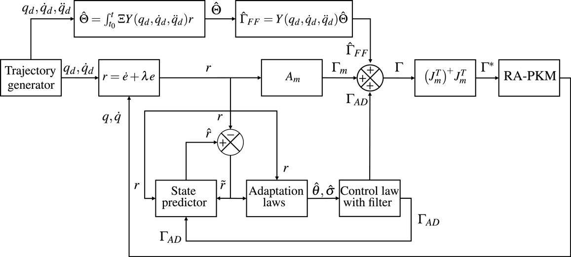
Figure 2. Block diagram of the proposed controller.

5. Experimental Validation of the Proposed Controller

To show the relevance of the proposed controller, real-time experiments have been conducted on ARROW robot. The experimental setup is illustrated in Figure 3 and the control scheme is developed using Simulink software from Mathworks Inc. The controller is compiled using the Real-Time Workshop toolbox before being loaded on the target PC. The latter is an industrial computer running xPC Target (also from Mathworks Inc.) in real-time with a sampling frequency of 5 kHz.

FIGURE 3

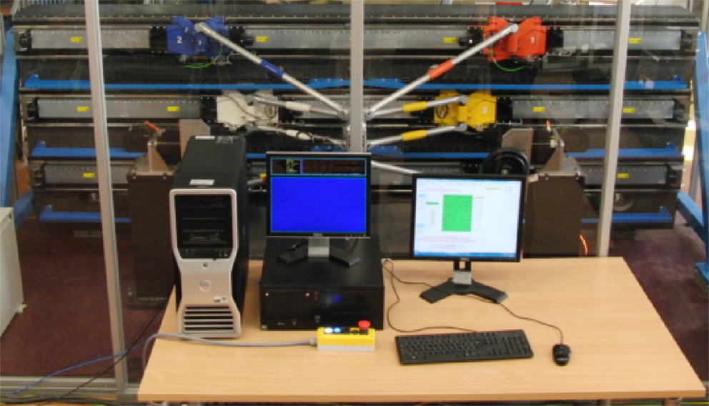
Figure 3. View of the experimental setup of ARROW PKM.

The moving platform of the robot has to perform several point-to-point displacements and rotations inside the workspace. The estimated parameters vector is initialized to 0 $\dot{\mathrm{\Theta }}\left(0\right)={\left[0,0,0,0\right]}^T$. The controller parameters of both controllers (the original ℒ₁ adaptive controller and the augmented one) are summarized in Table 2.

TABLE 2

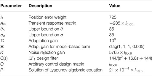
Table 2. Summary of the control parameters used in real-time experiments for both controllers.

A comparison between the ℒ₁ adaptive controller and the proposed augmented one in terms of joint tracking errors is illustrated in Figure 4. For clarity of the results, the plots were zoomed to the interval (Horowitz and Tomizuka, 1986; Khalil, 2002) seconds. It can be seen that the proposed model-based augmented controller clearly provides much better tracking than the original controller. Thanks to the model-based adaptive term, the controller successfully compensates the modeled non-linear dynamics with initially unknown parameters. It can also be seen that there exists an offset in the joint tracking errors in the case of the standard controller corresponding to the simple arms (i.e., q₁, q₂, q₅, and q₆). This is mainly due to the better handling of gravity effects in the proposed controller compared with the standard one. This result is further highlighted in Figure 5 where the Cartesian tracking errors are plotted. The plots are zoomed to the interval (Horowitz and Tomizuka, 1986; Khalil, 2002) seconds for clarity. An offset of the tracking errors corresponding to the y-axis (vertical axis) in the standard ℒ₁ adaptive controller, due to the previously mentioned reason. Since the robot is not equipped with external sensors, the Cartesian tracking errors e_c = [e_x, e_y, e_z, e_θ]^T ∈ ℝ⁴ were estimated using the following equation (Sartori Natal et al., 2015):

$e_c\left(t\right)=J_m^{+}{e}_q\left(t\right)$ (25)

where $e_q\left(t\right)\triangleq q_d\left(t\right)-q\left(t\right)$ is the joint tracking error vector. In order to quantify the enhancement brought by the proposed controller, the tracking performance is evaluated based on the root mean square of the tracking errors using the following criteria:

$\begin{array}{ll}\hfill {\text{RMS}}_J& =\sqrt{{\displaystyle \sum _{i=1}^6}\frac{1}{N}{\displaystyle \sum _{j=1}^N}{e}_{q_i}{\left(j\right)}^2}\end{array}$ (26)

$\begin{array}{ll}\hfill {\text{RMS}}_T& =\sqrt{\frac{1}{N}{\displaystyle \sum _{j=1}^N}{e}_x{\left(j\right)}^2+\frac{1}{N}{\displaystyle \sum _{j=1}^N}{e}_y{\left(j\right)}^2+\frac{1}{N}{\displaystyle \sum _{j=1}^N}{e}_z{\left(j\right)}^2}\end{array}$ (27)

$\begin{array}{ll}\hfill {\text{RMS}}_R& =\sqrt{\frac{1}{N}{\displaystyle \sum _{j=1}^N}{e}_{\mathrm{\theta }}{\left(j\right)}^2}\end{array}$ (28)

where $e_{q_i}$ is the tracking error of the i^th joint, e_x, e_y, and e_z are the Cartesian tracking errors of the x, y, and z-axis, respectively, and e_θ is the tracking error of the rotation of the moving platform. The obtained results are summarized in Table 3, where the improvements brought by the proposed controller are clearly highlighted. Indeed, the joint tracking errors were reduced by 79.4% and the Cartesian ones by up to 78.6%. The improvements of the tracking errors are achieved thanks to the better compensation of the non-linearities of the model. This means that the estimated model parameters do converge closer to their real values, otherwise the tracking performance would have been worst. Indeed, as it can be seen in Figure 6, the estimated parameters, initialized to 0, converge to their steady-state reported in Table 1. It is noticed that the rotational inertia of the platform is not adjusted immediately which is due to the pure translational motion at the beginning (i.e., t ∈ [0,6] s).

FIGURE 4

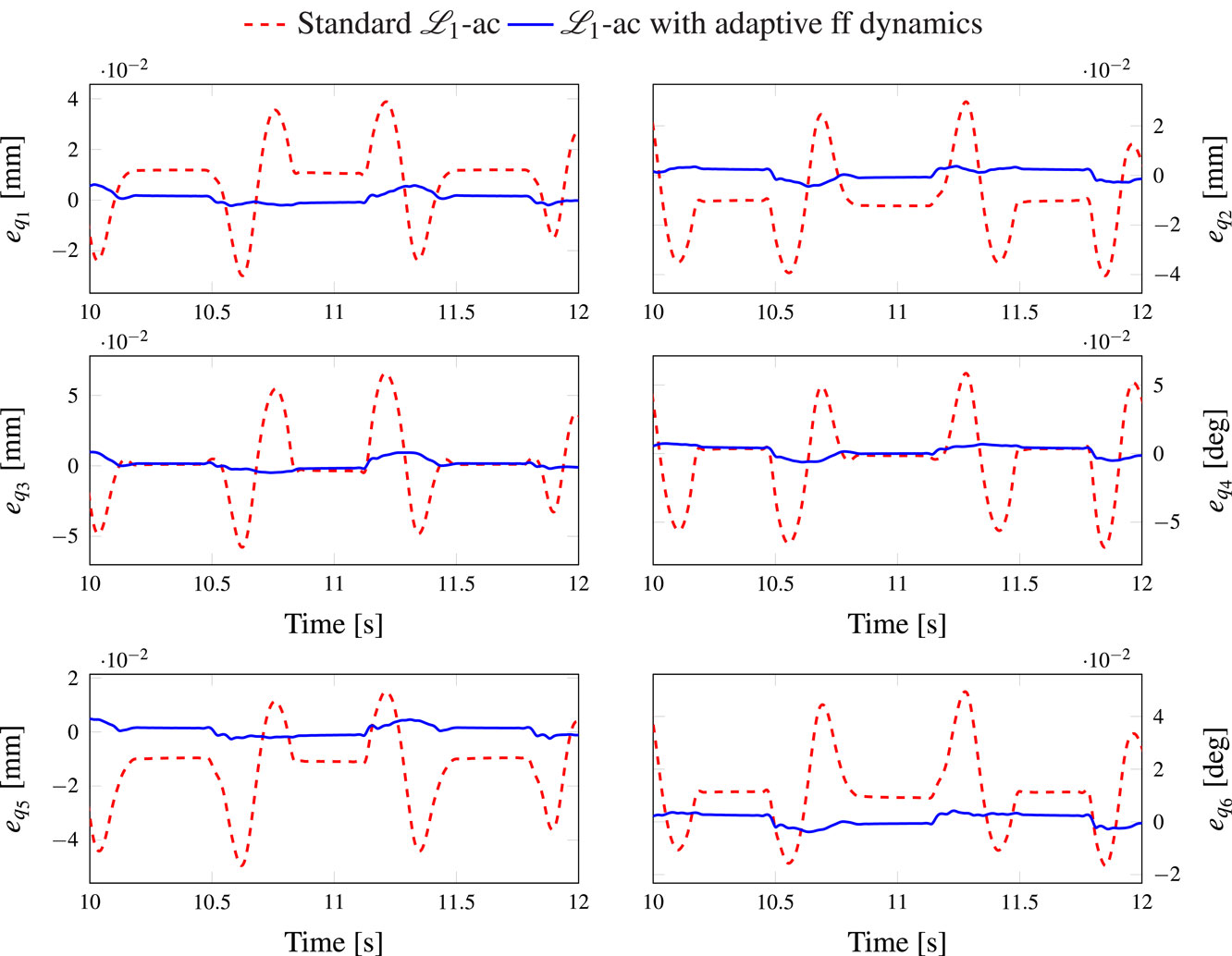
Figure 4. Evolution of the joint tracking errors versus time.

FIGURE 5

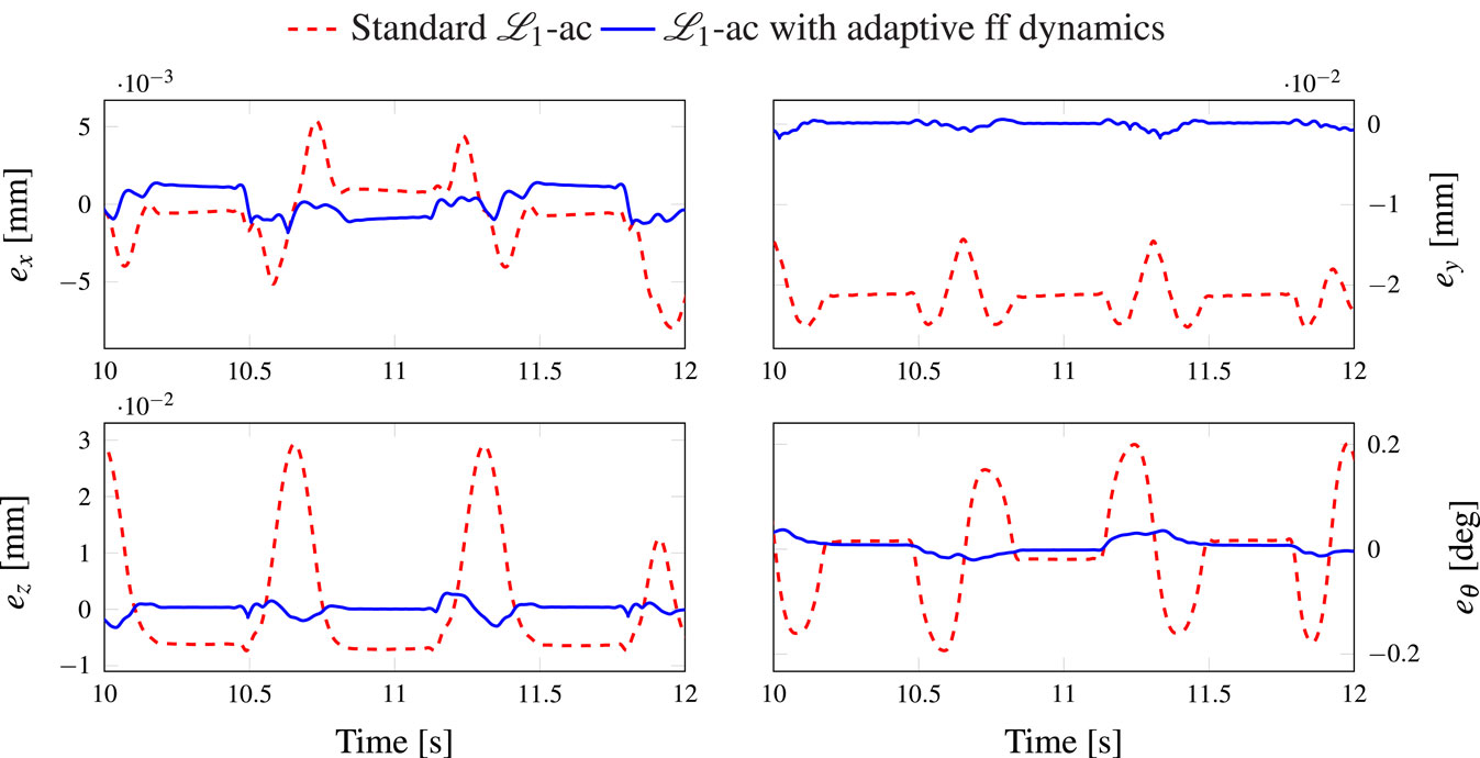
Figure 5. Evolution of the Cartesian tracking errors versus time.

TABLE 3

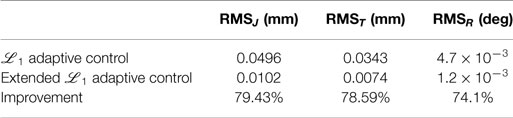
Table 3. Tracking performance comparison in terms of RMS errors.

FIGURE 6

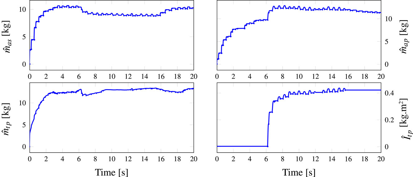
Figure 6. Evolution of the estimated dynamic parameters versus time.

Furthermore, since the model-based non-linearities are appropriately compensated, the estimated parameters forming the adaptive term Γ_AD(t) would be smaller in the case of the proposed controller. Indeed, these interesting results can clearly be observed in Figures 7 and 8, where we can see smaller amplitudes for the estimated parameters in the case of the proposed controller compared to the original one. This means that the structured uncertainties were better compensated by the proposed additional term and, hence, the ℒ₁ adaptive term should account for reduced non-linearities. Finally, the control input forces generated by both controllers are shown in Figure 9. Results can be viewed in the video available at the following URL: https://youtu.be/rCAocIWMfPs

FIGURE 7

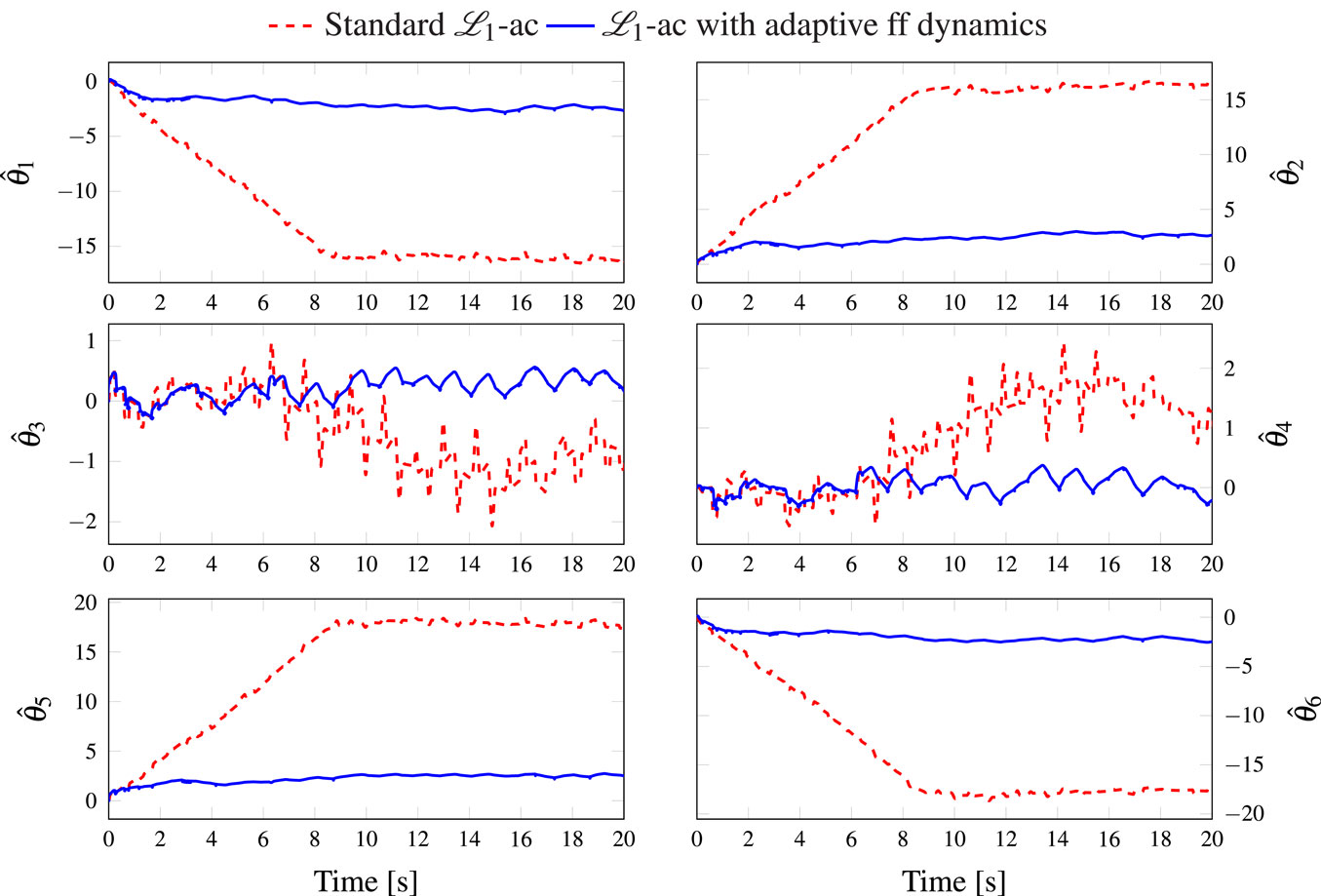
Figure 7. Evolution of the estimated function $\widehat{\mathbf{\theta }}$ versus time.

FIGURE 8

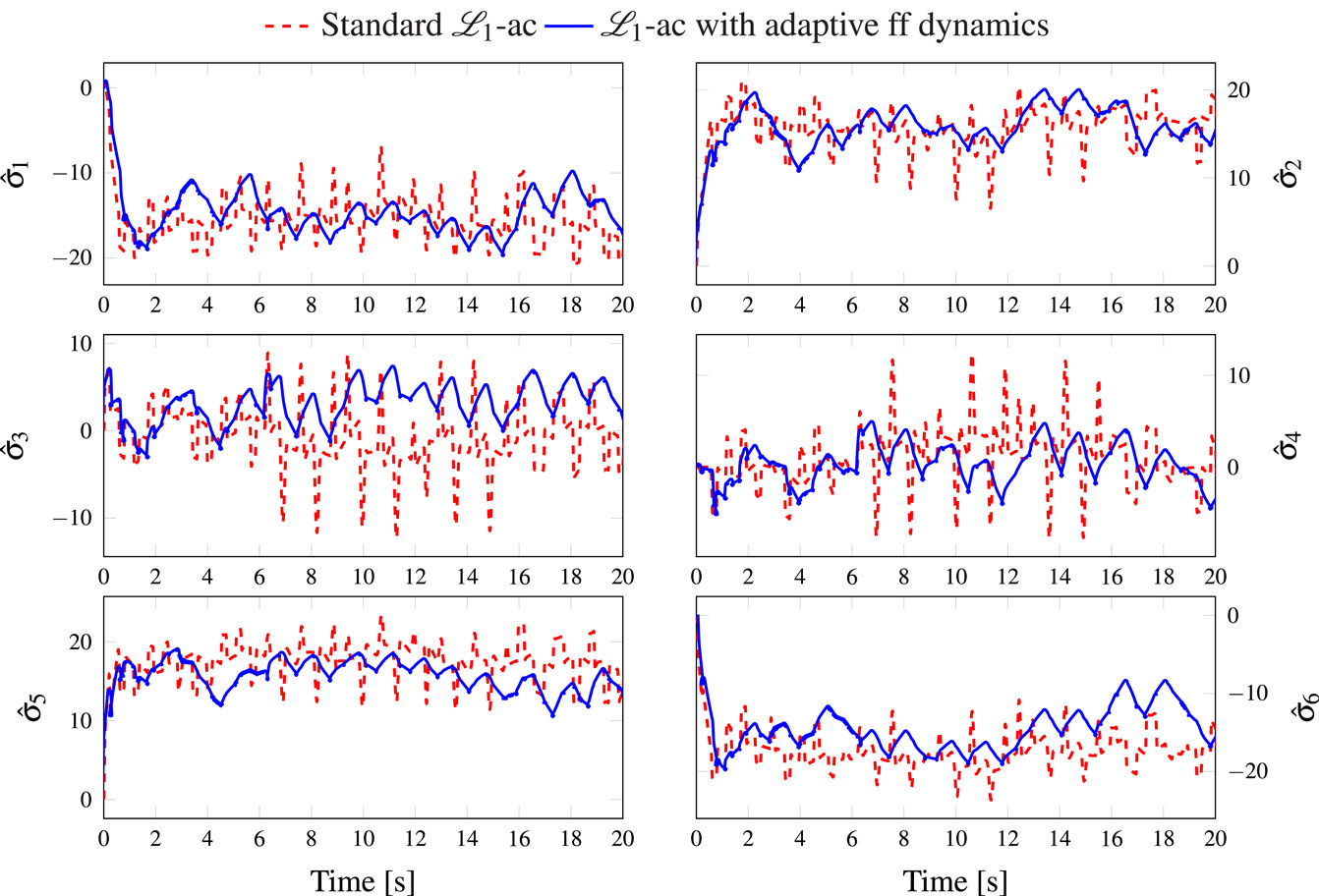
Figure 8. Evolution of the estimated function $\widehat{\mathbf{\sigma }}$ versus time.

FIGURE 9

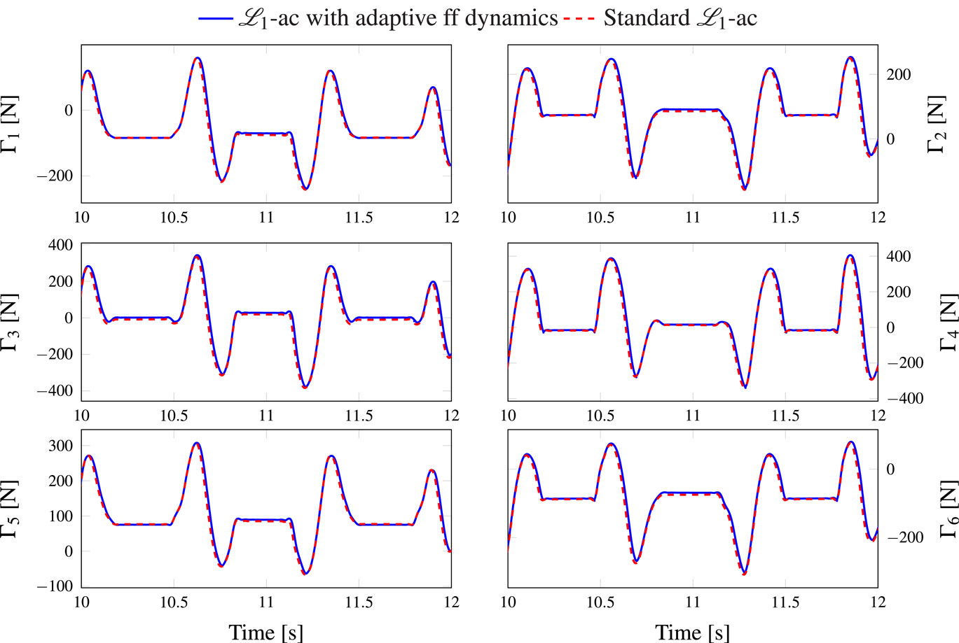
Figure 9. Evolution of the control inputs forces versus time.

6. Conclusion and Future Work

In this work, a new adaptive control scheme for mechanical manipulators based on ℒ₁ adaptive control theory is proposed. The original ℒ₁ adaptive controller is known for being model-free and for its robustness and fast adaptation qualities. Since in our case, a dynamic model of our redundantly actuated parallel manipulator is available, we have proposed to extend the original ℒ₁ adaptive controller by including dynamics knowledge in the control design. The motivation behind this proposition is to improve the tracking capabilities of the manipulator. Since the dynamics of the manipulator may be unknown or likely to vary during work conditions, we propose to make the additional model-based term adaptively adjust its parameters. Moreover, to deal with actuation redundancy, a projection of the control inputs was proposed in order to reduce the internal efforts that may have a negative effect on the control performance. Real-time experiments, conducted on a 4-DOF redundantly actuated parallel manipulator, demonstrate our claims. Indeed, a significant enhancement of the tracking performance was observed in both Cartesian and joint spaces. This work can be further extended by investigating other adaptive strategies for the model-based term and considering a real application where the robot is performing an industrial task. Another interesting scenario would be to consider an abrupt change in the platform mass due to payload handling for instance. Moreover, the tuning of the filter of the ℒ₁ adaptive controller remains an open problem that should be addressed in the future.

Conflict of Interest Statement

The authors declare that the research was conducted in the absence of any commercial or financial relationships that could be construed as a potential conflict of interest.

The Review Editor Francesco Pierri and the Associate Editor Filippo Arrichiello declared a current collaboration and the Associate Editor states that the process nevertheless met the standards of a fair and objective review.

Acknowledgments

This research was supported by the French National Research Agency (ANR) in the framework of the ARROW project (ANR-2011-BS3-006-01-ARROW).

Footnotes

1. ^BIBO: Bounded Input Bounded Output.
2. ^Parallel manipulators for which the number of actuators is equal to the number of degrees of freedom.

References

Andreas, M., and Hufnagel, T. (2011). “A projection method for the elimination of contradicting control forces in redundantly actuated PKM,” in Proceedings of IEEE International Conference on Robotics and Automation (ICRA’11) (Shanghai: IEEE), 3218–3223.

Google Scholar

Bennehar, M., Chemori, A., and Pierrot, F. (2014a). “A new extension of direct compensation adaptive control and its real-time application to redundantly actuated PKMs,” in IEEE/RSJ International Conference on Intelligent Robots and Systems (IROS’14) (Chicago, IL), 1670–1675.

Google Scholar

Bennehar, M., Chemori, A., and Pierrot, F. (2014b). “A novel rise-based adaptive feedforward controller for redundantly actuated parallel manipulators,” in IEEE/RSJ International Conference on Intelligent Robots and Systems (IROS’14) (Chicago, IL), 2389–2394.

Google Scholar

Bennehar, M., Chemori, A., and Pierrot, F. (2015). “L1 adaptive control of parallel kinematic manipulators: design and real-time experiments,” in IEEE International Conference on Robotics and Automation (ICRA’15) (Seattle, WA), 1587–1592.

Google Scholar

Cao, C., and Hovakimyan, N. (2006a). “Design and analysis of a novel ℒ₁ adaptive controller, part i: control signal and asymptotic stability,” in American Control Conference (ACC’06) (Minneapolis, MN), 3397–3402.

Google Scholar

Cao, C., and Hovakimyan, N. (2006b). “Design and analysis of a novel ℒ₁ adaptive controller, part ii: guaranteed transient performance,” in American Control Conference (ACC’06) (Minneapolis, MN), 3403–3408.

Google Scholar

Corbel, D., Gouttefarde, M., and Company, O. (2010). “Towards 100g with PKM is actuation redundancy a good solution for pick and place?,” in Proceedings of IEEE International Conference on Robotics and Automation (ICRA’10) (Anchorage, AK), 4675–4682.

Google Scholar

Craig, J. J., Hsu, P., and Sastry, S. S. (1987). Adaptive control of mechanical manipulators. Int. J. Robot. Res. 6, 16–28. doi: 10.1177/027836498700600202

CrossRef Full Text | Google Scholar

Dubowsky, S., and DesForges, D. T. (1979). The application of model-referenced adaptive control to robotic manipulators. J. Dyn. Syst. Meas. Control 101, 193–200. doi:10.1115/1.3426424

CrossRef Full Text | Google Scholar

Horowitz, R., and Tomizuka, M. (1986). An adaptive control scheme for mechanical manipulators – compensation of nonlinearity and decoupling control. J. Dyn. Syst. Meas. Control 108, 127–135. doi:10.1115/1.3143754

CrossRef Full Text | Google Scholar

Hovakimyan, N., and Cao, C. (2010). L1 Adaptive Control Theory: Guaranteed Robustness with Fast Adaptation. Philadelphia, PA: SIAM.

Google Scholar

Khalil, H. (2002). Nonlinear Systems, Vol. 3. Upper Saddle River, NJ: Prentice Hall.

Google Scholar

Markiewicz, B. (1973). Analysis of the Computed Torque Drive Method and Comparison with Conventional Position Servo for a Computer-Controlled Manipulator. Pasadena, CA: Jet Propulsion Laboratory, California Institute of Technology.

Google Scholar

Merlet, J. P. (2006). Parallel Robots, Second Edition. Dordrecht: Springer.

Google Scholar

Nguyen, K. D., Dankowicz, H., and Hovakimyan, N. (2013). “Marginal stability in ℒ₁ adaptive control of manipulators,” in Proceedings of the 9th ASME International Conference on Multibody Systems, Nonlinear Dynamics, and Control, Portland, OR.

Google Scholar

Ortega, R., and Spong, M. W. (1989). Adaptive motion control of rigid robots: a tutorial. Automatica 25, 877–888. doi:10.1016/0005-1098(89)90054-X

CrossRef Full Text | Google Scholar

Sadegh, N., and Horowitz, R. (1990). Stability and robustness analysis of a class of adaptive controllers for robotic manipulators. Int. J. Robot. Res. 9, 74–92. doi:10.1177/027836499000900305

CrossRef Full Text | Google Scholar

Sartori Natal, G., Chemori, A., and Pierrot, F. (2015). Dual-space control of extremely fast parallel manipulators: payload changes and the 100g experiment. IEEE Trans. Control Syst. Technol 23, 1520–1535. doi:10.1109/TCST.2014.2377951

CrossRef Full Text | Google Scholar

Shang, W., and Cong, S. (2010). Nonlinear adaptive task space control for a 2-dof redundantly actuated parallel manipulator. Nonlinear Dyn. 59, 61–72. doi:10.1007/s11071-009-9520-1

CrossRef Full Text | Google Scholar

Shayya, S. (2015). Towards Rapid and Precise Parallel Kinematic Machines. Ph.D. thesis, University of Montpellier, Montpellier.

Google Scholar

Shayya, S., Krut, S., Company, O., Baradat, C., and Pierrot, F. (2014). “A novel (3t-2r) parallel mechanism with large operational workspace and rotational capability,” in IEEE International Conference on Robotics and Automation (ICRA’14) (Hong Kong: IEEE), 5712–5719.

Google Scholar

Slotine, J., and Weiping, L. (1987). On the adaptive control of robot manipulators. Int. J. Robot. Res. 6, 49–59. doi:10.1177/027836498700600303

CrossRef Full Text | Google Scholar