In Search for the Neural Mechanisms of Individual Development: Behavior-Driven Differential Hebbian Learning

1. Introduction

Autonomy is a puzzling phenomenon both in the evolution of species and in individual development. Translating autonomy by “realizing an independent, self-determined development,” the question is how autonomy is grounded in the internal mechanisms of the individual, and even more interesting, what are the conditions for the emergence of this phenomenon. Common explanations postulate specific drives eliciting the emergence and subsistence of autonomous behavior. Examples are the selection pressure in evolution or intrinsic motivation in individual development. In recent years, such drives have been formulated in terms of objective functions ranging from the maximization of predictive information (Ay et al., 2008, 2012; Der et al., 2008; Martius et al., 2013) or empowerment (Klyubin et al., 2005; Salge et al., 2014), to the minimization of free energy (Friston, 2010), to the so-called time-loop error in the homeokinesis approach (Der, 2001; Der and Liebscher, 2002; Der and Martius, 2012), see also Prokopenko (2008, 2009) for more examples. Formulated at the level of behavior, those general principles may be translated into specific rules acting in the internal world of the agent.

Different from such a top-down way of thinking, this paper presents a bottom-up approach, claiming that there exist specific internal mechanisms that, while being unspecific for any task or survival strategy, per se have the ability to guide systems to self-determined activity. The hope to base the organization of behavior on local synaptic rules has been a major impact on research in neuroscience ever since the seminal work of Donald Hebb (1949). Hebb’s thinking was outstanding not only for its insight into the organization of the brain but also for its anticipation of modern ideas of self-organization, explaining how global order (behavior) can be based on local (synaptic) rules. The progress in neuroscience has provoked many variations and refinements of the original idea. For instance, the divergence problem is possibly counteracted by a synaptic scaling based on some homeostatic self-regulation mechanisms (Song et al., 2000; Turrigiano and Nelson, 2000, 2004; Carlson et al., 2013), and the spike-timing-dependent plasticity (STDP) (Gerstner et al., 1996; Markram et al., 1997; Bi and Poo, 1998) may overcome the problem of spurious associations induced by co-active neurons without causal relations. Also, there is some progress in reward-driven STDP invoking reinforcement learning and explaining several interesting experimental results (Fremaux et al., 2010; Kulvicius et al., 2010; Frémaux, 2013).

Nevertheless, with all the variations of the original law, the conclusion to the question how the neuronal mechanisms organize the behavior is still far from a convincing. In particular, unsupervised as they are, these neural mechanisms should be able to explain and realize the self-organized acquisition of sensorimotor competencies, at a basic level at least. I claim that this requires a more substantial change in the local rules and propose one possible solution in this paper.

Oriented at the original metaphor that synaptic development follows the simple law of “wiring” together what “fires together,” the new rule changes the synaptic connectivities driven by two incentives. On the one hand, the “wiring” is not driven by the firing activities of the neurons but by their rates of change. This is reminiscent of differential Hebbian learning studied in earlier work, see Kosko (1986), Klopf (1988), Roberts (1999), and Lowe et al. (2011). The advantage of differential over pure Hebbian learning for the self-organized behavior acquisition has been discussed in a concrete setting close to that of this paper in Der and Martius (2015). On the other hand, different from any Hebbian-like learning, the postsynaptic rate is not that of the neuron itself but is generated by a feedback chain from the external world the neuron is controlling. This link to the external world is the essential new feature and is what makes the new synaptic mechanism behaviorally relevant in an immediate way.

Neurorobotics is an ideal playground for testing this principle. With robots controlled by a neural network, one may expect not only new impacts for behavior generation in realistic settings but also get some feedback on the possible role of the new synaptic rule for biological systems. I will formulate this rule for the case of a flat sensorimotor loop as introduced in Section “Behavior-Driven Differential Hebbian Learning.” This minimalist control paradigm rests on the conviction that control should be less a prescription of what the robot is to do, but consists more in the excitation of specific modes emerging from the irreducible coupling of the mechanical system (robot + environment) with the nervous system. This whole-body paradigm is very close to the idea of morphological computation (Pfeifer and Gómez, 2009; Hauser et al., 2011, 2012; Pfeifer, 2012) but emphasizes more the role of an autonomous dynamics, given the morphology. The new unsupervised learning rule may be helpful in the realization of embodied intelligence that has found enormous interest in the last decade, see Pfeifer and Scheier (1999), Pfeifer and Bongard (2006), and Pfeifer et al. (2007) for excellent surveys and Ritter et al. (2009), Maycock et al. (2010, 2011), Mori and Kuniyoshi (2010), and Yamada et al. (2013) for applications, to name just a few.

This paper focuses on the close coupling between body, control, and environment in challenging physical settings, considering a spherical robot in Section “The Spherical,” a snake bot in Section “The Snake,” and a hexapod in Section “Discovering New Control Paradigms.” The examples demonstrate how the new synaptic mechanism induces a self-determined “search and converge” strategy in behavior space: starting from a dynamics germ these mechanisms elicit behavioral patterns, involving the whole body in tight conjunction with the internal mechanism. Additionally, well aware of the no-free-lunch theorem, I discuss in Section “Spontaneous Symmetry Breaking – the Pattern Behind the Patterns” the general phenomenon of spontaneous symmetry breaking, explaining how low-dimensional behavioral modes may emerge in high-dimensional systems seemingly out of nothing.

2. Behavior-Driven Differential Hebbian Learning

Let us start with formulating the rule in a concrete setting, considering generic robotic systems in physically realistic simulations. The robots are mechanical systems actuated by motors and equipped with a certain set of sensors. The controller, a neural network as described below, translates the sensor values observed in a certain time horizon into commands for the motors.

2.1. Synaptic Plasticity

Let us stipulate that the only information about its body and its interaction with the environment is given to the robot by its vector of sensor values x_t ∈ $\mathbb{R}$ⁿ. The controller is a neural network, mapping inputs x_t into the controls y_t ∈ $\mathbb{R}$^m. In the concrete application, the controller is a one-layer net of tanh neurons, described as

$y=g\left(\mathit{Cx}+h\right)$ (1)

where C is the m × n matrix of synaptic connections and g: $\mathbb{R}$^m → $\mathbb{R}$^m with g_i (z) = tanh (z_i). When learning this controller with a Hebbian law, the rate of change¹ of synapse C_ij would be proportional to the input x_j into the synapse j of neuron i multiplied by its activation y_i, i.e., ${\dot{C}}_{\mathit{ij}}$ ∝ y_ix_j. Differential Hebbian learning on its hand would use the rates of change, i.e., ${\dot{C}}_{\mathit{ij}}$ ∝ $\dot{y}$_i$\dot{x}$_j, see Kosko (1986), Klopf (1988), Roberts (1999), and Lowe et al. (2011). However, this must be modified in order to establish the contact with the external world. For that purpose, we need an internal representation for the relation between motor and sensor values. As we need only the rates of change, we relate the new (after a short time step) velocity vector ${\dot{x}}^{\prime }$ to the old velocities $\dot{x}$ and $\dot{y}$ as

${\dot{x}}^{\prime }=S\dot{x}+A\dot{y}+\mathrm{\eta }$ (2)

with the n × n matrix S and the n × m matrix A, η denoting the error in this relation. Let us introduce a new quantity $\dot{\tilde{y}}$ that is implicitly defined as

${\dot{x}}^{\prime }=S\dot{x}+A\dot{\tilde{y}}$ (3)

so that it incorporates the effect of the error, see Section “From Directed to Circular Causation” below for a more detailed discussion. The equation can be solved for $\dot{\tilde{y}}$ by using the (generalized) inverse of A. Including a decay term, we define the rate of change of the synaptic strength as

$\mathrm{\tau }{\dot{C}}_{\mathit{ij}}={\dot{\tilde{y}}}_i{\dot{x}}_j-C_{\mathit{ij}}$ (4)

where τ is the time scale for the synaptic dynamics. We will for the moment put the bias term h = 0, giving a law for its dynamics in equation (11) further below.

As we will see by the experiments, this extremely simple, purely deterministic rule [or its even more reduced counterpart given in equation (10) below] generates most complex behavior patterns as observed in the experiments. Metaphorically speaking, equation (4) is the internal law that enables the agent to realize a self-determined, independent development, establishing in this way its autonomy.

This new unsupervised learning rule is characterized by the metaphor of “chaining together what changes together.” As compared to Hebbian learning, this rule not only treats time in a more fundamental way (by considering rates of change instead of the pure firing rates) but includes in addition the chain of cause and effect in an inverse way from the behavior level down to the synaptic dynamics. This step grounds the behavior at the physical level deep in the internal world of the agent (at the level of the synaptic dynamics). Both features together make the system able to self-organize its behavior in close coupling between agent and environment. In view of these arguments, we will call the new rule behavior-driven differential Hebbian learning (BDDHL).

2.2. Empirical Gain Factor

The emergence of modes is contingent on the overall feedback strength of the sensorimotor loop. For controlling the latter, we introduce a gain factor for the neuron so that the action is defined as

$y=g\left(\mathrm{\kappa }\widehat{C}x+h\right)$ (5)

instead of equation (1), where the C matrix is obtained from equation (4) and Ĉ is normalized i.e., Ĉ = C /||C|| with ||C|| the (Frobenius) norm of C. κ is an empirical factor of order one that has to be chosen such that the overall feedback strength is slightly overcritical. In the subcritical region, the dynamics converges toward the resting behavior. In order to avoid numerical problems in this regularization procedure, we may either add a very weak noise to the vectors $\dot{\tilde{y}}$ and $\dot{x}$ in equation (4) or regularize the expression for Ĉ. In applications, an individual gain factor for each neuron is often more appropriate. This is strongly supported by neurophysiological findings on synaptic normalization (Carandini and Heeger, 2011), such as homeostatic synaptic plasticity (Turrigiano and Nelson, 2004), and the balanced state hypothesis (Tsodyks and Sejnowski, 1995; Monteforte and Wolf, 2010).

2.3. A First Discussion

Some obvious properties of that controller can easily be seen from following the signal flow in the closed sensorimotor loop (consider h = 0 for this argument). In each time step, the controller receives x and generates at first the postsynaptic potential z = Cx. By construction, Cx is a linear combination of velocities so that the controls y = g(Cx) also live in velocity space but are interpreted by the actuators as new target positions. So, the system can have a fixed point (FP) only if spatial positions (like the angle of a hinge joint) and the associated velocities (like the angular velocity of that hinge joint) are compatible over a time horizon set by τ. Trivially, there is a FP matching that condition if the controlled system is at rest so that ${\dot{x}}_t$ = 0 for t ≫ τ. In fact, with $\dot{x}$ = 0 we have C = 0 implying y = 0, i.e., all actuators are at their central positions (in the present setting and with h = 0). As the experiments show, if the gain factor is subcritical, this FP is even an attractor of the system with a wide basin.

However, the actual life of the system happens outside of that basin. In the behaving system, i.e., with velocities $\dot{x}$ ≠ 0, the target positions of the actuators are defined as a linear combination of these (past) velocities, which in general will be different from the values of x given by the current pose of the robot. This challenges a strong response of the system that on its hand is changing C what is producing new values for y, pulling x into new directions, and so on. This may lead to a self-amplification of modes if the feedback strength of the sensorimotor loop, as regulated by the gain factor κ, is sufficiently large.

2.4. From Directed to Circular Causation

The trick leading from equations (2) to (3) is the essential step for making the system able to self-organize. The common way of seeing a sensorimotor loop is to consider the actions y as the cause for the reaction of the system as reported by its sensor values. This postulates a signal flow from sensors to actions to new sensor values and so on. In this sense, the actions are seen as the causes for the sensorimotor dynamics. Of course, depending on contexts and given the complexity of the physical world, each action may generate a variety of effects. This is reflected by the η term in equation (2). Hence, the signal flow is still directed but not monocausal as it interweaves a specific cause with several effects.

Still, this corresponds to a directed causality. In this already pretty complex scenario, equation (3) introduces the auxiliary quantity $\dot{\tilde{y}}$, which incorporates implicitly the effects of the actions y. As $\dot{\tilde{y}}$ drives C, which on its hand determines the actions, eventually the actions are defined by their own effects. This is a clear case of circular causation in this complex dynamical system of interconnected causes and effects. With positive feedback strength in the sensorimotor loop, this principle elicits the self-organized behavior modes observed in the experiments.

2.5. Some Technical Details

Before going to the applications, let us note some details of the new rule. For a first reading, this part may be skipped.

2.5.1. Learning of the Response Matrix A

Inverse relations between sensor and motor spaces are notoriously difficult to find as they involve the physical response of the system to the applied controls. However, as demonstrated already in earlier work on homeokinesis (Der and Martius, 2012), a very coarse relation between these two worlds is entirely sufficient for the phenomenon of emerging whole-body modes. In the experiments of this paper, we put S = 0 so that A is updated in each time step as

$\dot{A}={\mathrm{\epsilon }}_A\left({\dot{x}}^{\prime }-A\dot{y}\right){\dot{y}}^{\mathsf{\text{T}}}$ (6)

where $\dot{y}$ is the rate of change of y in the current and ${\dot{x}}^{\prime }$ that of x in the next time step. The matrix A can be initialized either by hand, reflecting the known couplings between motor values and the corresponding sensor values, or can be found from a low-frequency and low-load motor babbling in an initiation phase of the development. Also, the inversion of A necessary to obtain the virtual controls $\dot{\tilde{y}}$ can be done with pseudoinverse techniques involving inversion only in motor space, given an arbitrary number of sensors. As an alternative, the inverse matrix can also be learned directly. Anyway, in most applications of this paper, the matrix A was simply taken as the unit matrix, hypothesizing a one-to-one sensor to motor coupling. Many technical details about these procedures may be found in Der and Martius (2012).

2.5.2. Explicit Expressions

The update rule generates the matrix C as a weighted average over the projectors on the past velocities in sensor space², i.e., switching to discrete times and using matrix notation, C_t being the controller matrix at time t

$C_t={\langle \dot{\tilde{y}}{\dot{x}}^{\mathsf{\text{T}}}\rangle }_0^t\approx \frac{1}{\mathrm{\tau }}{\displaystyle \sum _{t^{\prime }=0}^{t-\mathrm{1\hspace{0.17em}}}}{\dot{\tilde{y}}}_{t^{\prime }}{\dot{x}}_{t\prime }^{\mathsf{\text{T}}}{e}^{-\left(t-t^{\prime }\right)∕\mathrm{\tau }}+e^{-t∕\mathrm{\tau }}C\left(0\right)$ (7)

As the experiments show, the weighted average can be replaced with a simple windowing operation so that (assuming t ≫ τ)

$C_t=\frac{1}{\mathrm{\tau }}{\displaystyle \sum _{t^{\prime }=t-\mathrm{\tau }}^{t-1}}{\dot{\tilde{y}}}_{t^{\prime }}{\dot{x}}_{t\prime }^{\mathsf{\text{T}}}$ (8)

without losing much. In the experiments, τ ranges from 10 to 100 (roughly 0.2 to 2 s).

These explicit expressions also reveal a basic feature of the approach. Using equation (8) in equation (5) shows that the controller is given by a deterministic, explicit expression over the past sensor states. In fact, as ${\dot{\tilde{y}}}_t$ is a function of ${\dot{x}}_{t+1}$, we may rewrite equation (5) as

$y_t=K\left(x_t,x_{t-1},\dots ,x_{t-\mathrm{\tau }}\right)$ (9)

by approximating (with a convenient time scale) any ${\dot{x}}_{t^{\prime }}$ by $x_{t^{\prime }}-x_{t^{\prime }-1}$.

This demonstrates that the actions of the agent are defined by an explicit, fixed function of its recent sensor history. That this function is fixed, i.e., is not depending explicitly on time, does not mean that the behavior of the agent is fixed. Instead, as seen in the experiments, new experiences may well create new histories, leading to new behaviors creating new experiences and so on. Grounding the current behavior on its recent history is the qualitatively new feature of the approach that produces the observed variety of behaviors, seemingly out of nothing.

3. The Spherical

The Spherical is ideally suited for showing how BDDHL recognizes and amplifies dynamical structures in sensor space, creating thereby specific behavioral patterns in physical space. The spherical has a ball-shaped body and is driven by moving internal masses³, shifting thereby the center of gravity, see Figure 1. The control y_i defines the target position of the mass on its axis i. The only information the “brain” gets comes from three exteroceptive sensors, measuring the axis-orientation (with respect to the z-axis of the world coordinate system), and three proprioceptive sensors measuring the positions of the masses on their respective axes. Altogether the sensors give the robot only an extremely reduced information on its physical state.

FIGURE 1

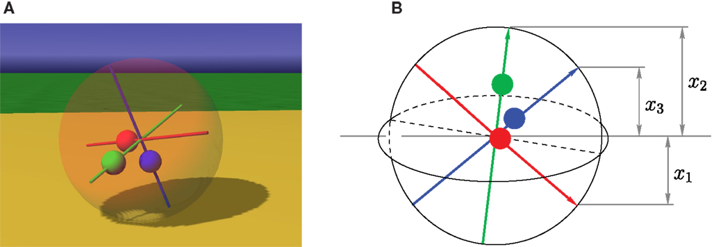
Figure 1. Spherical with axis-orientation sensors. (A) Screenshot from a simulation. The red, green, and blue masses are moved by actuators (linear motors) along the axes. (B) Schematic view of the robot with axis-orientation sensors (x_i), with x₁ < 0. The masses can interpenetrate each other but are otherwise “normal” physical objects. Proprioceptive sensors report the position of the masses on their respective axis.

I have chosen this machine because it demonstrates how BDDHL develops definite locomotion patterns starting from a dynamics germ. Without control, the physical behavior is quite simple if the weights are fixed in the center and the sphere is rolling on a 2-d plane. It becomes a little more complicated when, including friction and elasticity effects, opening the third dimension. With the masses outside of the center, the dynamics becomes kind of staggering and with an imposed motion of the masses the trajectory of the Spherical may become highly irregular, even if the controls are harmonic. This is similar to the Barrel case treated in some detail in Der and Martius (2012). So, any control scheme has to make its deal with these specific physical conditions. As the experiments show, the controller of this paper elicits without any knowledge of the physics very well-defined locomotion modes. Note that we use the notion of modes here as in physics, meaning that all degrees of freedom are coherently taking part in a behavior.

In the first set of experiments, the robot is moving on level ground that is elastic and has some friction to be as realistic as possible. In all simulations, we choose τ = 10, h = 0, κ = 1 and start with C = 0 so that all masses are in the center (least biased initialization). In the beginning, the robot is kicked by a mechanical force (an attracting force center marked by a red dot in the simulations) so that it starts rolling. This initial motion is rapidly picked up and amplified by BDDHL⁴, the most common mode being the rotation around one of the axes with the masses moving periodically on the other two axes. This mode is very stable against moderate external perturbations but can be switched into another of those modes by a very heavy kick, see video S1 on the supplementary materials site (Der, 2015).

When left alone, the future fate of the robot depends strongly on the learning rate ε_A of the response matrix A, see equation (6). This 6 × 3 matrix consists of two submatrices A^a and A^w mapping the control vector y to the axis orientation and the weight position sensors, respectively. In the experiments, we choose initially A^a = $\mathbb{I}$ and put all other matrix elements to 0. With ε_A below some critical value ε_crit, the emerging mode is stable for a very long time. With faster model learning, the system develops through a sequence of metastable rolling modes with widely differing characteristics, developing also a kind of lolloping mode and very fast locomotion as demonstrated in video S2 on the supplementary materials site (Der, 2015). In this way, the robot may be said to explore its behavioral spectrum of locomotion. More details are revealed by the parametric plots of the sensorimotor dynamics, showing a high degree of sensorimotor coordination when in the mode and a highly irregular behavior in the transition regions, see Figure 2.

FIGURE 2

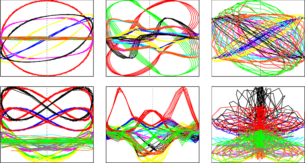
Figure 2. Parametric plots of the sensor and learning dynamics with robot on level ground. Top row: sensor values x_i(t) against x₀(t) when in a stable rolling mode (left), when in one of the fast modes (middle), and in the chaotic behavior when switching between modes (right). Bottom row: several of the C_ij(t) values against x₀(t) in the corresponding situations. See videos S1 and S2 on the supplementary materials site (Der, 2015).

In a next series of experiments, the robot is dropped into a large circular basin with an elastic, wavy ground, see video S3 on the supplementary materials site (Der, 2015). Dropped a little outside the center, the robot starts rolling downhill passively but, different from level ground, the robot first has to overcome an initial “orientation” phase with irregular motions, although there is no noise or any external stochasticity. After that, the robot goes into a stable mode running at constant height in the basin. Upon increasing ε_A a little, the sphere goes through several metastable states – running in orbits at a certain height – and leaves the basin after another increase in the learning rate ε_A, see also Figure 3.

FIGURE 3

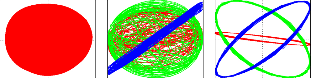
Figure 3. Motion of the Spherical in a basin. Trajectory as seen from above (left panel), parametric plot of the controls y_i(t) with i ∈ {1,2,3} vs. the sensor x₂(t) in the early “orientation” phase (middle) and later on when the robot is in an orbit of constant height in the basin (right).

Video S4 shows the behavior when five robots are started at the same time. Despite strong interactions between the individual robots, all five reach (essentially) the same orbit after some time. Two of the robots are seen to even return to their orbits after colliding. Later, the learning rate ε_A was increased making the robots to spiral higher and higher, eventually leaving the basin.

Interestingly, without knowing anything about the geometric structure of the world the robot is moving in, the emergence of the stable mode demonstrates that BDDHL, in a particular way, is sensitive to the agent–environment coupling (ACE). This will even be more obvious from the next example.

4. The Snake

Let us consider another machine – the Snake – in order to demonstrate the emergence of fundamental modes by the self-amplification process. This machine is completely different in physics as compared to the Spherical. Yet, we apply the same controller network, differing only in the number of motor neurons and the nature of the sensors, and apply the DHL rule as defined above, tuning nothing but the overall feed-back strength given by κ and the time scale τ. In this setting, mode generation will be established as a scalable phenomenon in the following experiments.

The Snake robot is composed of k capsules connected pairwise by a ball joint with two degrees of freedom (DOF) corresponding to two angles running from −ϕ to ϕ coded as y = −1 and y = 1. In every step, each angle is measured and reported as sensor value −1 < x_i < 1. The motors driving each DOF receive a target value for the desired joint angle in the next step. The translation into the physical forces (like the torques of a joint) is done by an embedded PID controller tuned such as to simulate the elasticity of muscles. Driven by the physical forces acting between the individual elements, this elasticity effect makes the true angles to differ vastly from their target values once the robot is in full activity. Let me emphasize that all the information the robot has comes from these proprioceptive sensors giving no information about the physical situation of the robot in its environment.

4.1. Simplifying the Learning Rule

Despite this high physical complexity, the experiments show that the forward model, given by the matrix A, can be kept very simple – it turns out that it is sufficient to learn the model by a simple, low-frequency motor babbling when the joints are without load (as it would be in 0 gravity space without obstacles and/or ground contact). In the current setting, this reduces the forward model to A = $\mathbb{I}$. As it turns out, the concomitant model learning can be switched off altogether so that equation (4) becomes

$\mathrm{\tau }{\dot{C}}_{\mathit{ij}}={\dot{x}}_i^{\prime }{\dot{x}}_j-C_{\mathit{ij}},$ (10)

where $\dot{x}$ = $\dot{x}$(t) and ${\dot{x}}^{\prime }$ = $\dot{x}$(t + 1) are the rates of change of the joint angles as reported by the sensors. This simplified BDDHL rule is what was used in the experiments discussed in the following, i.e., in both the Snake and in the Hexapod case, as well as in many other applications done so far. Together with the normalization procedure [equation (5)], this extremely simple rule was found in the applications to elicit within minutes (real time) an amazing variety of sensorimotor patterns without any scaffolding from outside.

In the experiments, in all cases, the controller was initialized in the least biased setting, meaning C = 0 and h = 0 so that all actuators are in their central positions. In the Snake case, this means that the body is completely stretched. This situation corresponds to the trivial attractor, where the system is at rest so that, initially, the system must be started by a mechanical impact on the robot body⁵ or by adding some noise to the sensor values.

4.2. Emerging Locomotion Patterns

In a first set of experiments, we put the snake on even ground giving it a kick in the very beginning and whenever it comes to rest. What we observe is that the system develops right from the outset after a very short time (seconds) a collective mode with all degrees of freedom changing coherently. What kind of mode may develop in this initial phase depends on the initial kick and/or the sequence of kicks one is applying in order to get the system going. In the experiments, we see two qualitatively different modes emerging, either a meandering motion like crawling with a certain velocity over ground, or a kind of siderolling, reminiscent of the sidewinding motion known from snakes in sandy deserts, which has also been reproduced by artificial evolution (Prokopenko et al., 2006), see videos S5 and S6 on the supplementary materials site (Der, 2015). Figure 4 gives a few examples of emerging motion patterns together with the C matrices. Obviously, the latter show distinct structures in close relation to the motion patterns. This will be discussed in Section “Spontaneous Symmetry Breaking – the Pattern Behind the Patterns” below.

FIGURE 4

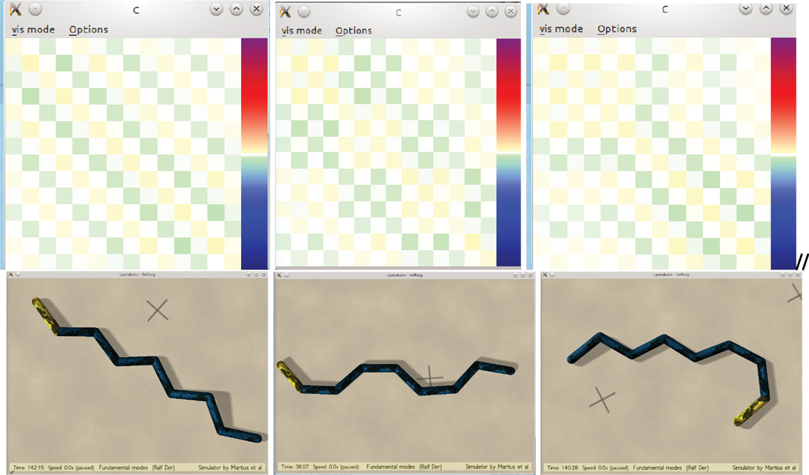
Figure 4. The controller matrix C (above) with the Snake in various stable siderolling locomotion modes (below).

These emerging locomotion modes in general are metastable but may last for very long times if there are no external perturbations. The system can be forced by mechanical kicks to leave the current mode, but is engaging into another mode after some time, often just a few seconds real time, see video S6 on the supplementary materials site (Der, 2015). In the transitional phase, the system is highly irregular, as is best seen by considering the parametric plots in Figure 5.

FIGURE 5

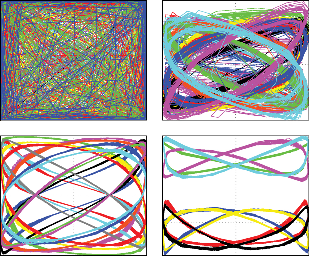
Figure 5. Parametric plots demonstrating the formation of a mode and the emerging dimensionality reduction. The first three panels depict the sensor values x_i(t) with i = 0. 13 against the controller output y₆(t) in a time interval of 500 steps (10 s). Top left depicts the behavior in the transition phase between two modes with fully developed chaos, top right depicts the formation of a new mode, and bottom left corresponds to the fully developed mode demonstrating the high degree of sensorimotor coordination. The time between these three phases is about 1 min. The bottom right depicts the behavior of some of the matrix elements of C vs. y₆, demonstrating the tight correlation of the synaptic dynamics with the behavior of the physical system.

4.3. The Constitutive Role of the Agent–Environment Coupling

Another point of interest is the active role of the agent–environment coupling in generating the behavior. This is demonstrated by two effects. On the one hand, modes may switch in a definite way by interacting with the environment. When colliding with a wall, or any other obstacle, the Snake will change actively its direction of motion so that it kind of reacts to the collision with the boundary, see videos S8 and S9. Note that there is no contact sensor or the like, the Snake simply reacts to the different coupling with the environment it experiences at the boundary. In the collision, the velocities of the joint angles go to 0 (due to the friction between body and obstacle) giving rise to a mode switching.

On the other hand, the modes are a direct consequence of the agent–environment coupling. This becomes most obvious when this coupling is switched off. Let us consider an experiment with the robot in a stable mode (rolling or crawling). As video S7 on the supplementary materials site (Der, 2015) shows that the modes decay rapidly once the gravity is temporarily being switched off so that the contact with the ground is lost. So, the coupling with the ground is an inexorable ingredient of the mode formation and existence. As an explanation, we note that, given the friction and elasticity of the ground, the different degrees of freedom strongly interact by the forces exerted on each other when moving on the ground. More details on this so-called physical cross-talk effect may be found in Der (2014). This physical cross-talk has an immediate influence on the velocities of the sensor values, which feeds back to the behavior via the C matrix in a synchronizing way.

Videos S8 and S9 demonstrate another effect of the agent–environment coupling: when colliding with a wall or any other obstacle, the Snake experiences a strong physical cross talk by the reactive forces exerted on the joints. This leads, via the induced synaptic dynamics, to a collective reorganization of the system that expresses itself as a reversion of the locomotion velocity. Note that there is nothing like a contact sensor reporting the collision. Instead, the emerging reaction is a pure whole system effect, generating a variety of reactions depending on the circumstances.

4.4. Emergent Dimensionality Reduction

Another important feature is the emergent reduction of dimensionality when converging to the mode. At a more qualitative level, the parametric plots are a convincing indication that the system is confined to a low-dimensional manifold at least in a blurred sense, see Figure 5. Interestingly, we also observe that the life time of a mode is directly related to the structure of the parametric plot. The more stable a mode is, the cleaner are the orbits of the sensor values in the parametric plot and the closer is the system to moving on a low-dimensional manifold. Moreover, the life time of the modes is observed to be directly related to the velocity of the Snake over ground. So, the higher the velocity of locomotion, the cleaner the plot. This may be explained by the assumption that the synchronization via the forces across the ground is best if the DOFs cooperate in producing an effective locomotion pattern.

On a quantitative level, there are first results (Martius and Olbrich, 2013) that the dimension of the manifold is a little above two, stipulating an appropriate coarse graining. Note that the phase space of the constrained physical system is of 2 × (6 + 2K) dimensions, with K + 1 the number of segments and K = 8 in the video.

5. Discovering New Control Paradigms

The last example is to demonstrate the “creative” power of BDDHL to discover new ways of controlling high-dimensional systems. For this purpose, let us modify our system by adding a rule for the dynamics of the bias vector h ∈ $\mathbb{R}$^m in equation (1). The idea is that the bias dynamics drives the neurons toward their region of maximal sensitivity. With the bipolar tanh neurons used in this paper a convenient choice is

$\dot{h}=-{\mathrm{\epsilon }}_{h}y,$ (11)

where y is the output vector of the controller neurons as defined by equation (5) and ε_h is the update rate to be chosen by hand. This dynamics is of particular interest in hysteresis systems as discussed in earlier work (Der and Martius, 2012).

For a discussion, let us consider still another machine, the so-called Hexapod, see Figure 6. Apart from its morphology, the robot is constructed in its functionality like the Snake robot, with synaptic dynamics given by equation (10) and the bias dynamics of equation (11). As with the Snake, we may put A ≈ $\mathbb{I}$ and consider first the case of a diagonal controller matrix C = c$\mathbb{I}$. Then, the system dynamics is split into individual, decoupled feedback loops. As discussed in Der and Martius (2012) and Der (2014) and others, if h = 0 and the coupling strength c is overcritical, each of these loops has two FPs. Considering only the six vertical shoulder joints, the system has 2⁶ FPs corresponding to each joint angle either high or low.

FIGURE 6

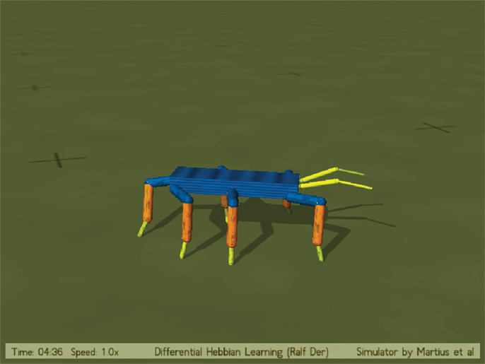
Figure 6. The Hexapod.

If the h dynamics is switched on, each of those individual circuits becomes a so-called hysteresis oscillator producing a periodic oscillation. Interestingly, these non-linear oscillators have a high tendency to synchronize so that collective locomotion and other dynamical patterns are created, see for instance the so-called Armband robot in Der and Martius (2012) and the videos under playfulmachines.com.

5.1. Experiments – From Motion Germs to Organized Behavior

Now let us drive the parameters of the controller by equation (10) together with the bias dynamics equation (11). Depending on both the starting conditions of the mechanical system and of the controller, we get a vast variety of possible behavior patterns. In all experiments, we start with the least biased controller using C = 0 and h = 0 so that y = 0, corresponding to the central position of all actuators. Jumping patterns emerge in a natural way if we drop the robot from a certain height. With the trunk in a horizontal pose, the robot hits ground with all its legs at the same time. Due to the muscle-like flexibility of the motor-joint system, the robot responds with a damped vertical oscillation. Similar to the Spherical case treated in Section “The Spherical,” the BDDHL controller picks up and amplifies this motion germ so that the robot almost immediately executes a more or less stable hopping motion, see video S10 on the supplementary materials site (Der, 2015).

Jumping with all four legs into the air simultaneously is called stotting or pronking and is observed in many quadruped animals, with gazelles in particular, see Figure 7. It seems not to be observed in hexapods but we will call the emerging motion patterns also a stotting behavior. With quadrupeds, there must be some evolutionary advantage for the development of this behavior but it seems not to be clear what exactly that is. Nevertheless, it is interesting that BDDHL automatically develops such a behavior without any rewards or evolutionary pressure. I will give an argument in terms of the symmetry group considerations that may explain the preferential emergence of this behavior, see Section “Spontaneous Symmetry Breaking – the Pattern Behind the Patterns” below. Moreover, the frequency of this stotting motion pattern can be regulated by the value of ε_h in a certain range.

FIGURE 7

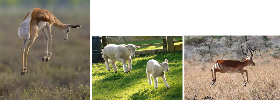
Figure 7. Just for fun? Stotting behavior in animals. The animals spring into the air vertically with all feet lifting simultaneously. The evolutionary advantage seems to be unclear. Authors: Yathin Sk (left), Pam from near Matamata (middle), Rick Wilhelmsen (right), all pictures from Wikimedia commons.

Shaping the pattern is also possible by playing with the time scale parameter τ of equation (4) and the gain factor of the neurons κ. By varying these parameters while the robot is behaving, the robot can also be brought into a forward jumping behavior, sometimes called a bound gait (Yamasaki et al., 2013), see video S11.

5.2. Stotting and Collective Hysteresis

The jumping pattern gets an explanation if we look at the emerged structure of the controller matrix C that defines the behavior together with the bias dynamics of equation (11). As illustrated by Figure 8, behaviors are identifiable by the geometrical pattern of their control matrix. It is interesting to see that and how (see below) BDDHL develops control structures that are intimately related to the physical properties, like the dynamics and morphology, of the mechanical system it is controlling.

FIGURE 8

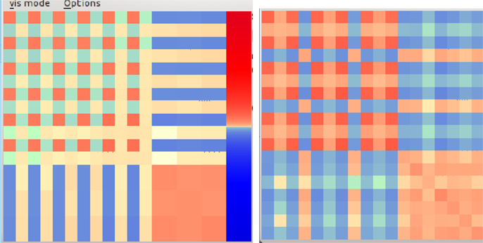
Figure 8. Structure of the control matrix when in the jumping motion pattern (left). The upper left 12 × 12 matrix, referring to the shoulder joints, shows a regular chess board-like pattern. In a later, more complex motion (right) the chess board pattern has been resolved into a more complex geometrical structure, indicating a more intricate cooperation between the various degrees of freedom. Quite generally, different modes correspond to different geometric patterns of the control matrix.

In the stotting case, it is essentially the synchronous motion of the vertical shoulder joints that generates the jumps. This is directly reflected by the large values of the corresponding sensor to motor coupling elements of the upper left 12 × 12 matrix. Numerically, we observe that all matrix elements involving the up–down shoulder joints, i.e., C(0,0), C(0,2), …, C(10,10) are self-regulating toward roughly the same value c = 0.2. Ignoring all the other (much smaller elements) for the moment and putting h = 0, the system has two stable FPs corresponding to all legs either up or down simultaneously.

This is easily explained by comparing the present situation with that of the individual hysteresis loops (see above) generating 2⁶ FPs if c > 1. In the present situation, a hysteresis loop is generated by the cooperation between the individual feedback loops. In fact, summing the feedback strengths of all loops contributing to one motor output gives just the slightly overcritical feedback 6 × c ≈ 1.2 for the signal flow through that neuron. So, all the feedback loops are intermingled in a systematic way and when including the h dynamics, a strongly synchronized motion is emerging. Importantly, as the videos show, the repeated contact with the ground helps stabilizing this synchrony by the muscle-like flexibility of the motor-joint system. This is another example of the constitutive role of the agent–environment coupling.

We may call the emerging control scheme a whole-body hysteretic controller and note that this new way of controlling emerged directly from the BDDHL rule under the given physical initialization. With more complex C matrix patterns, see Figure 8, more complex motion patterns are readily produced by this new control paradigm. This will be investigated in a later paper. It is also to be noted that the pronounced systematics in the structure of the controller matrix can also be used for editing behaviors ex post.

Many other interesting motion patterns can be seen by the videos on the emergence and decay of locomotion patterns at the beginning of the supplementary material page (Der, 2015).

6. Spontaneous Symmetry Breaking – The Pattern Behind the Patterns

The role of symmetries of the system for the pertinent motion patterns has been extensively studied in the literature, see Schöner et al. (1990), Collins and Stewart (1993), Strogatz and Stewart (1993), Golubitsky et al. (1998, 1999), van der Weele and Banning (2001), Golubitsky (2012), and Tero et al. (2013). In those works, gaits are driven by central pattern generators (CPGs) that are constructed of non-linear oscillators. The CPGs may be considered as open-loop controllers imposing their rhythms on the mechanical system as was the case in the earlier models (Collins and Stewart, 1993; Strogatz and Stewart, 1993; Golubitsky et al., 1998, 1999), or they may respond to the interaction with the body, closing the sensorimotor loop, see Tero et al. (2013).

6.1. Geometric Symmetries

Systems of coupled oscillators are well known from classical mechanics and can be analyzed to some degree. As the investigations show, the various gaits can be associated with the symmetries of the controlled system. In particular, one can study the role of the invariance of the body’s geometry against permutations. With quadrupeds, these are the invariance against right–left or back–front permutations, e.g., in the case of the Hexapod, the corresponding symmetry group is given by the permutations of all legs (assuming complete forward backward symmetry). In the periodically driven systems, there is still the invariance against time shifting by the period duration T.

In those papers, starting from the most general group comprising the maximum number of invariance, hierarchies of symmetry groups were constructed by progressively reducing the set of invariance. Special behaviors, such as different locomotion patterns, can be associated with a definite symmetry group. For instance, stotting may be associated with the group of maximum symmetry. Transitions between gaits can be associated with symmetry breaking bifurcations (Collins and Stewart, 1993; van der Weele and Banning, 2001). So, the approach leads to natural hierarchies of gaits, ordered by symmetry, and to natural sequences of gait bifurcations.

In the bifurcation scenario discussed in those papers, symmetry breaking was induced by changing the controller parameters, such as the amplitude and frequency of the driving force in Collins and Stewart (1993) and van der Weele and Banning (2001), from outside: when crossing the bifurcation point, the system becomes instable and the system state jumps into one of the emerging alternatives. With BDDHL, we have a self-referential system (Der and Martius, 2012), a dynamical system that changes its parameters by itself, driven by the BDDHL mechanism.

6.2. Symmetries of the Physical Dynamics

The geometric symmetries are only the upper level of the whole spectrum of symmetries associated with the physical dynamics of the mechanical system. For a sketch, let us consider the robot in its least biased initialization as discussed above, corresponding to the central position of all actuators (with corrections due to the load on the joints). When linearizing around that state, the resulting dynamical system is characterized by a bunch of symmetries like the invariance against inverting the sign of joint angles. These symmetries are approximate since they can be perturbed by non-linearities, the actions of the controller, and the interaction with the environment and/or other body parts. Yet, starting from an unspecific dynamics germ, we observe the emergence of motion patterns reflecting the original symmetries of the physical system to a high degree [the principle of parsimonious symmetry breaking, see Der and Martius (2013) and Der (2014)].

When starting with the least biased initialization, i.e., C = 0 and h = 0, these broken symmetry patterns are emerging in the interaction process of the controller with the body and the environment. This has been demonstrated by the emerging structures of the controller matrix C, see Figures 4 and 8, which directly reflect the permutation symmetries of the body. Why is that? The decisive point in this scenario is the fact that the BDDHL mechanism is invariant against just the involved symmetry groups. Considering the explicit expressions for the C matrix given in equations (7) and (8), this is most obvious in the case of sign inversion and permutations of the sensor–motor pair x,y. A more involved symmetry is given by rotations of the sensor–motor space. For a discussion, let us consider the case A = $\mathbb{I}$ as discussed with the Snake and the Hexapod. With x → Ux where U is a rotation matrix so that U^𝖳 = U⁻¹, we obtain Cx →UCx so that, according to equation (1), y → Uy. This establishes the (approximate) invariance of the system against (x, y) → (Ux, Uy) (if the non-linearities can be ignored, as is the case in the starting phase of a mode out of the least biased initialization).

Having stated that, why do the symmetry broken motion patterns emerge? The point now is that BDDHL, with an overcritical value of the global feedback strength (controlled by the gain factor κ), destabilizes the system so that an initial perturbation is amplified. As this amplification process is (approximately) invariant under the operations of the symmetry group, the emerging dynamics stays in the largest symmetry group that is compatible with the initial perturbation. This is like a kind of conservation rule for the symmetry group the system is in. This argument explains why the system goes for the largest group, the stotting in the case of the Hexapod: the larger the group, the larger is the probability that the initial perturbation is consistent with the group, in the sense that it is approximately invariant under the operations of the group.

The initial perturbation can also be realized by some noise that is invariant under the operations of the group. Then, the perturbation is fully unspecific so that the symmetry breaking is truly spontaneous. Otherwise, as already mentioned, when kicking the system by an external impact, the perturbation is not fully unspecific, one even can usher the system into a specific symmetry group, like in the case of the Snake with its emerging crawling or siderolling modes. This is another interesting feature of the BDDHL approach.

7. Conclusion

This paper proposes a new synaptic law for the organization of behavior that replaces Hebb’s original metaphor of “wiring” together what “fires together” by “chaining together” what “changes” together, linking the motor neurons by a feedback chain to the behavior in the physical world consisting of body and environment. This feedback chain is the essential new feature of the proposed synaptic rule and is what makes the synaptic dynamics behaviorally relevant in an immediate way.

In applications to a number of complex robots, it was demonstrated that neurocontrollers with that new rule elicit an amazing variety of complex behavior patterns, contingent on the specific embodiment and the agent–environment coupling. The patterns have been shown to directly reflect the symmetries of the body and the agent–environment coupling. In particular, a physical system with many degrees of freedom like the Snake is seen to self-organize into definite locomotion patterns without rewarding or prestructuring the system in any way. This example also showed the tremendous reduction of dimensionality emerging in the controlled systems. For instance, in the examples with the Snake, the constrained physical systems live in a phase space of up to 40 dimensions. Yet, the controlled system converges within seconds toward a (blurred) low-dimensional manifold, hosting the definite locomotion pattern.

The results suggest new ways for robotics. With the self-organization ability realized by the BDDHL rule, robots can be driven into different behaviors by external influences and can switch between behaviors just by interaction with the environment or a human trainer. This also opens new ways for a kinesthetic teaching as will be detailed in a later paper. BDDHL realizes a “search and converge” strategy in behavior space that can be guided by just two metaparameters – the time scale τ of the synaptic dynamics and the gain factor κ of the controller neurons. Different from most search strategies, BDDHL realizes a self-determined search, a deterministic process with actions being defined as a plain function of the sensor values (over the recent past) so that all behaviors are repeatable and utilizable as building blocks in behavioral architectures. This is an advantage over other approaches, such as homeokinesis (Der and Liebscher, 2002; Der and Martius, 2012), which also produce interesting behaviors but are more inclined to search and less to a convergence toward definite (though metastable) behaviors.

Neural networks often are blamed for the opacity of the solutions found by a learning procedure. Interestingly, this is different with the present approach. In the experiments with both the Snake and the Hexapod, definite structures of the synaptic matrix were observed, revealing transparent relations between emerging behavior and control structure. So, given the pronounced, behavior-related structure in the controller matrix, the emerging behaviors can be understood and even be edited to shape behaviors into desired directions.

The presented results may also have some impact on biology. It was demonstrated that an extremely simple synaptic rule can, contingent on the morphology and the agent–environment coupling, elicit a vast variety of behavioral patterns that may have an immediate evolutionary advantage. On a speculative level, this may be considered as a new factor in natural evolution. It is commonly assumed in natural evolution that new behaviors are the result of a mutation in morphology accompanied by an appropriate mutation of the controller so that the probability of selection is the product of two (very small) probabilities. Had nature discovered the BDDHL rule, new species with new behaviors could emerge just by mutations of the morphology, trusting that BDDHL will drive the modified system to new, fitness relevant modes of behavior. As proposed by Baldwin (Baldwin, 1896; Weber and Depew, 2003), such new behaviors, reoccurring in every generation, could be made permanent eventually by another mutation freezing the behavior. It would be interesting to look for indications of the new synaptic plasticity in living systems.

Let me conclude with a few words on the question in what sense are the emerging behaviors autonomous? The nature of autonomy is still widely debated, see, for instance Di Paolo (2005) and Bertschinger et al. (2008). My attitude is a very modest one, just stating that autonomy is large if the agent unfolds a rich spectrum of different behavioral patterns, driven by an internal law that is as free as possible on the wishes and intentions of its designer. This freedom postulate is fulfilled almost ideally with the rules of equation (4) or (10) as the behavior of the agent is entirely determined by a universal law that is formulated at the synaptic level, two levels deeper than that of the behavior, and it is formulated entirely in terms of the sensor values the robot has generated by its actions in its recent past. So, in this setting, there is no room for the designer to sneak its intentions in. However, quantifying the richness of the behavior spectrum is an open question so that, in this sense, autonomy remains in the eyes of the beholder.

Author Contributions

All research is done by the author.

Conflict of Interest Statement

The author declares that the research was conducted in the absence of any commercial or financial relationships that could be construed as a potential conflict of interest.

Acknowledgments

The author gratefully acknowledges the hospitality in the group of Nihat Ay at the Max Planck Institute for Mathematics in the Sciences, Leipzig, and many helpful and clarifying discussions with Nihat Ay, Georg Martius, and Keyan Zahedi.

Supplementary Material

Videos and further details may be found at http://robot.informatik.uni-leipzig.de/research/supplementary/NeuroAutonomy/

Footnotes

1. ^We use the common overdot notation for rates of change or velocities.
2. ^The solution of the matrix differential equation $\mathrm{\tau }\dot{C}\left(t\right)=R\left(t\right)-C\left(t\right)$ is used as $C\left(t\right)=\frac{1}{\mathrm{\tau }}{\int }_0^t\mathrm{\hspace{0.17em}R}\left(t\prime \right)e^{-\left(t-t\prime \right)/\tau }\mathit{dt}\prime +e^{-t/\tau }\mathrm{\hspace{0.17em}C}\left(0\right)$. The discrete expression is obtained by taking the Riemannian sum, which is exact if τ →∞.
3. ^Collisions of those masses are ignored in the simulations.
4. ^Provided the parameter κ is large enough.
5. ^In the simulator, this is realized by a force center marked by a red dot in the videos.

References

Ay, N., Bernigau, H., Der, R., and Prokopenko, M. (2012). Information-driven self-organization: the dynamical system approach to autonomous robot behavior. Theory Biosci. 131, 161–179. doi:10.1007/s12064-011-0137-9

PubMed Abstract | CrossRef Full Text | Google Scholar

Ay, N., Bertschinger, N., Der, R., Güttler, F., and Olbrich, E. (2008). Predictive information and explorative behavior of autonomous robots. Eur. Phys. J. B 63, 329–339. doi:10.1140/epjb/e2008-00175-0

CrossRef Full Text | Google Scholar

Baldwin, J. M. (1896). A new factor in evolution. Am. Nat. 30, 441–451, 536–553. doi:10.1086/276428

CrossRef Full Text | Google Scholar

Bertschinger, N., Olbrich, E., Ay, N., and Jost, J. (2008). Autonomy: an information theoretic perspective. BioSystems 91, 331–345. doi:10.1016/j.biosystems.2007.05.018

PubMed Abstract | CrossRef Full Text | Google Scholar

Bi, G. Q., and Poo, M. M. (1998). Synaptic modifications in cultured hippocampal neurons: dependence on spike timing, synaptic strength, and postsynaptic cell type. J. Neurosci. 18, 10464–10472.

PubMed Abstract | Google Scholar

Carandini, M., and Heeger, D. J. (2011). Normalization as a canonical neural computation. Nat. Rev. Neurosci. 13, 51–62. doi:10.1038/nrn3136

PubMed Abstract | CrossRef Full Text | Google Scholar

Carlson, K. D., Richert, M., Dutt, N., and Krichmar, J. L. (2013). “Biologically plausible models of homeostasis and stdp: stability and learning in spiking neural networks,” in Neural Networks (IJCNN), The 2013 International Joint Conference on (Dallas, TX: IEEE), 1–8. doi:10.1109/IJCNN.2013.6706961

CrossRef Full Text | Google Scholar

Collins, J. J., and Stewart, I. N. (1993). Coupled nonlinear oscillators and the symmetries of animal gaits. J. Nonlinear Sci. 3, 349–392. doi:10.1007/BF02429870

CrossRef Full Text | Google Scholar

Der, R. (2001). Self-organized acquisition of situated behaviors. Theory Biosci. 120, 179–187. doi:10.1078/1431-7613-00039

CrossRef Full Text | Google Scholar

Der, R. (2014). “On the role of embodiment for self-organizing robots: behavior as broken symmetry,” in Guided Self-Organization: Inception, Volume 9 of Emergence, Complexity and Computation, ed. M. Prokopenko (Heidelberg: Springer), 193–221.

Google Scholar

Der, R. (2015). Supplementary Materials to Neuroautonomy. Available at: http://robot.informatik.uni-leipzig.de/research/supplementary/NeuroAutonomy/

Google Scholar

Der, R., Güttler, F., and Ay, N. (2008). “Predictive information and emergent cooperativity in a chain of mobile robots,” in Proceedings Eleventh International Conference on the Simulation and Synthesis of Living Systems. eds S. Bullock, J. Noble, R. A. Watson, and M. A. Bedau (Winchester, UK: MIT Press).

Google Scholar

Der, R., and Liebscher, R. (2002). “True autonomy from self-organized adaptivity,” in Proc. Workshop Biologically Inspired Robotics (Bristol).

Google Scholar

Der, R., and Martius, G. (2012). The Playful Machine – Theoretical Foundation and Practical Realization of Self-Organizing Robots. Berlin: Springer.

Google Scholar

Der, R., and Martius, G. (2013). “Behavior as broken symmetry in embodied self-organizing robots,” in Proceedings of the Twelfth European Conference on the Synthesis and Simulation of Living Systems. eds P. Liò, O. Miglino, G. Nicosia, S. Nolfi, and M. Pavone (Taormina: MIT Press), 601–608.

Google Scholar

Der, R., and Martius, G. (2015). Novel plasticity rule can explain the development of sensorimotor intelligence. Proc. Natl. Acad. Sci. U.S.A. 112, E6224–E6232. doi:10.1073/pnas.1508400112

PubMed Abstract | CrossRef Full Text | Google Scholar

Di Paolo, E. A. (2005). Autopoiesis, adaptivity, teleology, agency. Phenomenol. Cogn. Sci. 4, 429–452. doi:10.1007/s11097-005-9002-y

CrossRef Full Text | Google Scholar

Frémaux, N. (2013). Models of Reward-Modulated Spike-Timing-Dependent Plasticity. Ph.D thesis, IC, Lausanne.

Google Scholar

Fremaux, N., Sprekeler, H., and Gerstner, W. (2010). Functional requirements for reward-modulated spike timing-dependent plasticity. J. Neurosci. 30, 13326–13337. doi:10.1523/JNEUROSCI.6249-09.2010

CrossRef Full Text | Google Scholar

Friston, K. (2010). The free-energy principle: a unified brain theory? Nat. Rev. Neurosci. 11, 127–138. doi:10.1038/nrn2787

CrossRef Full Text | Google Scholar

Gerstner, W., Kempter, R., Hemmen, J. V., and Wagner, H. (1996). A neuronal learning rule for sub-millisecond temporal coding. Nature 383, 76–81. doi:10.1038/383076a0

PubMed Abstract | CrossRef Full Text | Google Scholar

Golubitsky, M. (2012). Animal gaits and symmetry. Spring 2012 Meeting of the APS Ohio-Region Section, Vol. 57 (Columbus, OH). Available at: http://meetings.aps.org/link/BAPS.2012.OSS.D1.3

Google Scholar

Golubitsky, M., Stewart, I., Buono, P.-L., and Collins, J. (1998). A modular network for legged locomotion. Physica D 115, 56–72. doi:10.1016/S0167-2789(97)00222-4

CrossRef Full Text | Google Scholar

Golubitsky, M., Stewart, I., Buono, P.-L., and Collins, J. (1999). Symmetry in locomotor central pattern generators and animal gaits. Nature 401, 693–695. doi:10.1038/44416

PubMed Abstract | CrossRef Full Text | Google Scholar

Hauser, H., Ijspeert, A. J., Füchslin, R. M., Pfeifer, R., and Maass, W. (2011). Towards a theoretical foundation for morphological computation with compliant bodies. Biol. Cybern. 105, 355–370. doi:10.1007/s00422-012-0471-0

CrossRef Full Text | Google Scholar

Hauser, H., Ijspeert, A. J., Füchslin, R. M., Pfeifer, R., and Maass, W. (2012). The role of feedback in morphological computation with compliant bodies. Biol. Cybern. 106, 595–613. doi:10.1007/s00422-012-0516-4

PubMed Abstract | CrossRef Full Text | Google Scholar

Hebb, D. O. (1949). The Organization of Behavior: A Neuropsychological Theory. New York, NY: Wiley.

Google Scholar

Klopf, A. H. (1988). A neuronal model of classical conditioning. Psychobiology 16, 85–125.

Google Scholar

Klyubin, A. S., Polani, D., and Nehaniv, C. L. (2005). “Empowerment: a universal agent-centric measure of control,” in Congress on Evolutionary Computation (Edinburgh: IEEE), 128–135. doi:10.1109/CEC.2005.1554676

CrossRef Full Text | Google Scholar

Kosko, B. (1986). “Differential Hebbian learning,” in AIP Conference Proceedings, Vol. 151, 277–282.

Google Scholar

Kulvicius, T., Kolodziejski, C., Tamosiunaite, M., Porr, B., and Wörgötter, F. (2010). Behavioral analysis of differential Hebbian learning in closed-loop systems. Biol. Cybern. 103, 255–271. doi:10.1007/s00422-010-0396-4

PubMed Abstract | CrossRef Full Text | Google Scholar

Lowe, R., Mannella, F., Ziemke, T., and Baldassarre, G. (2011). “Modelling coordination of learning systems: a reservoir systems approach to dopamine modulated Pavlovian conditioning,” in Advances in Artificial Life. Darwin Meets von Neumann. Vol. 5778. eds G. Kampis, I. Karsai, and E. Szathmáry (Berlin Heidelberg: Springer), 410–417.

Google Scholar

Markram, H., Lübke, J., Frotscher, M., and Sakmann, B. (1997). Regulation of synaptic efficacy by coincidence of postsynaptic APs and EPSPs. Science 275, 213–215. doi:10.1126/science.275.5297.213

PubMed Abstract | CrossRef Full Text | Google Scholar

Martius, G., Der, R., and Ay, N. (2013). Information driven self-organization of complex robotic behaviors. PLoS ONE 8:e63400. doi:10.1371/journal.pone.0063400

PubMed Abstract | CrossRef Full Text | Google Scholar

Martius, G., and Olbrich, E. (2013). “Quantifying emergent behavior of autonomous robots (extended abstract),” in Workshop on Artificial Life in Massive Data Flows, ECAL 2013 (Taormina).

Google Scholar

Maycock, J., Dornbusch, D., Elbrechter, C., Haschke, R., Schack, T., and Ritter, H. (2010). Approaching manual intelligence. KI Künstliche Intelligenz 24, 287–294. doi:10.1007/s13218-010-0064-9

CrossRef Full Text | Google Scholar

Maycock, J., Essig, K., Haschke, R., Schack, T., and Ritter, H. (2011). “Towards an understanding of grasping using a multi-sensing approach,” in International Conference on Robotics and Automation (ICRA) (Saint Paul).

Google Scholar

Monteforte, M., and Wolf, F. (2010). Dynamical entropy production in spiking neuron networks in the balanced state. Phys. Rev. Lett. 105, 268104. doi:10.1103/PhysRevLett.105.268104

PubMed Abstract | CrossRef Full Text | Google Scholar

Mori, H., and Kuniyoshi, Y. (2010). “A human fetus development simulation: self-organization of behaviors through tactile sensation,” in Development and Learning (ICDL), 2010 IEEE 9th International Conference on (Ann Arbor: IEEE), 82–87.

Google Scholar

Pfeifer, R. (2012). “Morphological computation” – self-organization, embodiment, and biological inspiration,” in International Joint Conference IJCCI 2012. Vol. 577. eds K. Madani, C. A. Dourado, A. Rosa, and J. Filipe (Barcelona) p. 110.

Google Scholar

Pfeifer, R., and Bongard, J. C. (2006). How the Body Shapes the Way We Think: A New View of Intelligence. Cambridge, MA: MIT Press.

Google Scholar

Pfeifer, R., and Gómez, G. (2009). “Morphological computation – connecting brain, body, and environment,” in Creating Brain-Like Intelligence: From Basic Principles to Complex Intelligent Systems (Lecture Notes in Computer Science), eds S. Bernhard, K. Edgar, S. Olaf, and R. Helge (Berlin: Springer), 66–83.

Google Scholar

Pfeifer, R., Lungarella, M., and Iida, F. (2007). Self-organization, embodiment, and biologically inspired robotics. Science 318, 1088–1093. doi:10.1126/science.1145803

PubMed Abstract | CrossRef Full Text | Google Scholar

Pfeifer, R., and Scheier, C. (1999). Understanding Intelligence. Boston, MA: MIT Press.

Google Scholar

Prokopenko, M. (2009). Information and self-organization: a macroscopic approach to complex systems. Artif. Life 15, 377–383. doi:10.1162/artl.2009.Prokopenko.B4

CrossRef Full Text | Google Scholar

Prokopenko, M. (ed.) (2008). Foundations and Formalizations of Self-Organization. Berlin: Springer.

Google Scholar

Prokopenko, M., Gerasimov, V., and Tanev, I. (2006). “Evolving spatiotemporal coordination in a modular robotic system,” in From Animals to Animats 9, Volume 4095 of LNCS, eds S. Nolfi, G. Baldassarre, R. Calabretta, J. Hallam, D. Marocco, J.-A. Meyer, and D. Parisi (Berlin: Springer), 558–569.

Google Scholar

Ritter, H., Haschke, R., and Steil, J. J. (2009). “Trying to grasp a sketch of a brain for grasping,” in Creating Brain-Like Intelligence: From Basic Principles to Complex Intelligent Systems (Lecture Notes in Computer Science). eds S. Bernhard, K. Edgar, S. Olaf, and R. Helge (Berlin: Springer), 84–102.

Google Scholar

Roberts, P. D. (1999). Computational consequences of temporally asymmetric learning rules: I. Differential Hebbian learning. J. Comput. Neurosci. 7, 235–246. doi:10.1023/A:1008910918445

PubMed Abstract | CrossRef Full Text | Google Scholar

Salge, C., Glackin, C., and Polani, D. (2014). “Empowerment-an introduction,” in Guided Self-Organization: Inception (Heidelberg: Springer), 67–114.

Google Scholar

Schöner, G., Jiang, W. Y., and Kelso, J. S. (1990). A synergetic theory of quadrupedal gaits and gait transitions. J. Theor. Biol. 142, 359–391. doi:10.1016/S0022-5193(05)80558-2

PubMed Abstract | CrossRef Full Text | Google Scholar

Song, S., Miller, K. D., and Abbott, L. F. (2000). Competitive Hebbian learning through spike-timing-dependent synaptic plasticity. Nat. Neurosci. 3, 919–926. doi:10.1038/78829

PubMed Abstract | CrossRef Full Text | Google Scholar

Strogatz, S. H., and Stewart, I. (1993). Coupled oscillators and biological synchronization. Sci. Am. 269, 102–109. doi:10.1038/scientificamerican1293-102

CrossRef Full Text | Google Scholar

Tero, A., Akiyama, M., Owaki, D., Kano, T., Ishiguro, A., and Kobayashi, R. (2013). Interlimb neural connection is not required for gait transition in quadruped locomotion. arXiv preprint arXiv:1310.7568.

Google Scholar

Tsodyks, M. V., and Sejnowski, T. (1995). Rapid state switching in balanced cortical network models. Netw. Comput. Neural Syst. 6, 111–124. doi:10.1088/0954-898X_6_2_001

CrossRef Full Text | Google Scholar

Turrigiano, G. G., and Nelson, S. (2000). Hebb and homeostasis in neuronal plasticity. Curr. Opin. Neurobiol. 10, 358–364. doi:10.1016/S0959-4388(00)00091-X

PubMed Abstract | CrossRef Full Text | Google Scholar

Turrigiano, G. G., and Nelson, S. B. (2004). Homeostatic plasticity in the developing nervous system. Nat. Rev. Neurosci. 5, 97–107. doi:10.1038/nrn1327

CrossRef Full Text | Google Scholar

van der Weele, J. P., and Banning, E. J. (2001). Mode interaction in horses, tea, and other nonlinear oscillators: the universal role of symmetry. Am. J. Phys. 69, 953. doi:10.1119/1.1378014

CrossRef Full Text | Google Scholar

Weber, B. H., and Depew, D. J. (2003). Evolution and Learning: The Baldwin Effect Reconsidered. Cambridge, MA: MIT Press.

Google Scholar

Yamada, Y., Fujii, K., and Kuniyoshi, Y. (2013). “Impacts of environment, nervous system and movements of preterms on body map development: fetus simulation with spiking neural network,” in Development and Learning and Epigenetic Robotics (ICDL), 2013 IEEE Third Joint International Conference on (Osaka: IEEE), 1–7.

Google Scholar

Yamasaki, R., Ambe, Y., Aoi, S., and Matsuno, F. (2013). “Quadrupedal bounding with spring-damper body joint,” in Intelligent Robots and Systems (IROS), 2013 IEEE/RSJ International Conference on (Tokyo: IEEE), 2345–2350.

Google Scholar