Comparison Study of Subtropical Mode Waters in the World Ocean

Introduction

The structure of the subtropical thermocline has fascinated theoretical and observational physical oceanographers alike for many years, because it is perhaps one of the most prominent aspects of the ocean. To understand the mechanisms of formation and maintenance of such ocean structure is a classical, but still an active research topic (Rhines and Young, 1982a,b; Luyten et al., 1983; Marshall, 2000; Marshall et al., 2001; Dewar et al., 2005). One effective approach is to focus on water masses that are associated with distinctive ocean structures. We can consider physical mechanisms that form ocean structure by examining/investigating the formation, advection and dissipation of those water masses.

Mode water is a type of water mass, characterized by uniform water properties with large volume and thus corresponds to the specific mode of the volumetric distribution on the temperature and salinity bivariate plane (Worthington, 1959; Speer and Forget, 2013). Hanawa and Talley (2001) categorizes mode waters into three categories according to their distribution areas. Type 1 mode waters are subtropical mode waters (STMW), associated with the subtropical western boundary current (WBC). Type 2 mode waters are located eastern part of subtropical gyre. Type 3 mode waters are mainly located in the subpolar area. Mode waters prevail in the upper layer of the world ocean with a large horizontal distribution of over several hundred thousand square kilometers and several hundred meter thickness (Hanawa and Talley, 2001).

Distribution of mode water has been examined from potential vorticity dynamics point of view. One of the epoch-making theories to understand the upper ocean structure is proposed by Luyten et al. (1983), known as ventilated thermocline theory. They suggest that the upper ocean structure can be understood as a layer model where potential vorticity is conserved once the water is subducted into the interior ocean. The theory concerning homogenization of potential vorticity, known as homogenization theory, is proposed by Rhines and Young (1982a,b) to treat the western shadow zone of the ventilated thermocline theory. Huang and Russell (1994) calculates the upper ocean structure with continuous stratification and wind stress data based on the ventilated thermocline theory and the homogenization theory. Following the above theoretical hypothesis (Rhines and Young, 1982a,b; Luyten et al., 1983), mode waters have been regarded as an important water mass to evaluate the distribution of potential vorticity on an isopycnal layer using observation data (Talley, 1988; McCarthy and Talley, 1999; Suga et al., 2004).

STMW is a distinctive ocean structure as a result of ocean-atmosphere interaction in the mid-latitude WBC system. A deep winter mixed layer develops in the western part of the subtropical gyre because warmer water carried by the WBC is subjected to severe winter cooling by the polar air outbreaks from the continents (Hanawa and Talley, 2001; Speer and Forget, 2013). The STMW distribution area, at least partly, coincides with the recirculation gyre of WBC. Therefore, although, there are many mechanisms involved, the nature of STMW is fundamentally related to the characteristics of the WBC, winter cooling and the recirculation gyre.

STMW is regarded as an important water mass for several reasons. Since STMW is the remnant of the winter mixed layer, STMW preserves the temperature anomaly which reflects the intensity of winter cooling and acts as memory of the signal of climate variation (Yasuda and Hanawa, 1997; Oka and Qiu, 2011). STMW transmits these memories to the interior ocean below the winter mixed layer through the subduction process (Marshall et al., 1993) and can affect the sea surface temperature in the following winter, known as the reemergence mechanism (Alexander et al., 1999). Reemergence is presented as one of the key mechanisms influencing the inter-decadal ocean-atmospheric variability in the North Pacific (Sugimoto and Hanawa, 2005, 2007) and in the North Atlantic (Timlin et al., 2002; Cassou et al., 2007). STMW may play a role in nutrient supply in the subtropical gyre. Sukigara et al. (2011) suggests that North Pacific STMW (NPSTMW; Masuzawa, 1969) possibly provides nutrients to the euphotic zone of the western part of subtropical gyre. On the other hand, Palter et al. (2005) suggests that North Atlantic STMW (NASTMW; Worthington, 1959) prevents the upwelling of nutrient rich water from the deeper levels.

In recent years, intensive observation campaigns have been carried out to study WBC system both in the North Pacific and the North Atlantic: Kuroshio Extension System Study (KESS) in 2003–2008 for the North Pacific and CLIvar MOde water Dynamics Experiment (CLIMODE) in 2005–2007 for the North Atlantic. The KESS project involves a three dimensional meso-scale eddy-resolving mooring array and large number of profiling float measurements (http://uskess.whoi.edu). The CLIMODE field campaign incorporates two times winter-time field campaigns across the Gulf Stream (Marshall et al., 2009; http://climode.org/index.html). Along with the KESS and CLIMODE projects, Kelly et al. (2010) and Kwon et al. (2010) review similarities and dissimilarities of ocean—atmosphere interaction in the mid-latitude WBC system between the North Pacific and the North Atlantic. A goal of their reviews is intend to better understand the WBC system by synthesizing the KESS outcomes and CLIMODE outcomes.

STMWs in each basin (the North Pacific, the North Atlantic, the South Pacific, the South Atlantic, and the Indian Ocean) have different characteristics in terms of thickness, volume, temperature, and salinity. STMWs are formed under different conditions such as the strength of winter cooling, strength of WBC, precipitation, evaporation, and separation latitude of the WBC (Roemmich and Cornuelle, 1992; Hanawa and Talley, 2001). Since there are complex interactions between dynamics and thermodynamics and between ocean and atmosphere in the mid-latitude WBC system (Kelly et al., 2010), it is difficult to evaluate every single process that forms the characteristics of STMW. By comparing characteristics of STMWs and formation conditions in different basins, we could assess gross effect of these mechanisms that form characteristics of STMWs. In this way, we could obtain implications which factor may or may not determine the STMW characteristics. Highlighting similarities and dissimilarities of STMWs may facilitate to transfer our understandings on STMW formation, advection, and dissipation mechanisms from one basin to another. Although “comparison study of STMW” could be a useful approach, only qualitative comparison has been partially discussed (Roemmich and Cornuelle, 1992; Kelly et al., 2010; Kwon et al., 2010; Kobashi and Kubokawa, 2011). The bottom line issue is that we do not have uniform criteria to extract STMWs in different basins. As a result, we cannot quantify characteristics of STMW in different basins.

This paper has two objectives. The first objective is to propose a uniform criterion of STMW in order to quantify the horizontal and vertical spatial structures of STMW in different basins. The second objective is to demonstrate the benefit of “comparison study of STMW” by highlighting similarities and dissimilarities of STMWs and investigating major factors that influence the vertical structure of STMW. The contents of this paper are as follows. Second Section describes the data and methods used in this study. Third Section is the result section. We first introduce a newly defined common criterion of STMW. We then describe the horizontal and vertical spatial structure of STMW using the common criterion. Major factors that influence the STMW thickness are also investigated. In Fourth Section, we discuss the role of WBC forming thicker STMW from a viewpoint of the potential vorticity dynamics, and the unique vertical structure of STMW in the South Atlantic. Fifth Section gives a summary and conclusion.

Data and Methods

Data Sets

The temperature and salinity climatology data of HydroBase version 2 (Lozier et al., 1995; MacDonald et al., 2001; Kobayashi and Suga, 2006) is used in this study. The HydroBase monthly climatology is provided on a 1° × 1° spatial grid at standard levels (0, 10, 20, 30, 50, 75, 100, 125, 150, 200, 250, 300, 400, 500, 600, 700, 800, 900, 1000 m, and so on). Since the HydroBase climatology is constructed by isopycnal averaging using temperature and salinity data, representation of ocean structure near the strong density fronts, e.g., the Kuroshio, the Gulf Stream and the Antarctic Circumpolar Current tends to be better than depth averaging hydrographic datasets. Note that Hydrobase version 2 is primary based on historical ship-based hydrographic data. It does not contain most of the Argo data. This means that number of profiles in the Southern Hemisphere is lower than that of the Northern Hemisphere, and original hydrographic data is centered around 1990's. Moreover, since gridded data is provided at the standard levels, it only captures large vertical structure of more than 100 m in the upper ocean.

Standard depth data are interpolated to 10-m vertical intervals using Akima's shape-preserving local spline (Akima, 1970). The vertical temperature gradient (dT/dz) and vertical salinity gradient (dS/dz) at a certain grid is calculated as a first difference between vertically adjacent grid points below and above (their depth difference is 20 m). Potential vorticity (PV; m⁻¹s⁻¹) is also calculated from density difference in the same way using the equation below (Equation 1).

$\begin{array}{l}PV=\frac{f}{\rho }\frac{\partial \rho }{\partial z}\end{array}$

Where f is the coriolis parameter (s⁻¹) and ρ is potential density (kg m⁻³) reference to surface. The coriolis parameter in Southern Hemisphere is multiplied by −1. The monthly climatology data of July, August, and September are averaged to calculate the summer mean ocean structure in the Northern Hemisphere and those of January, February, and March are averaged to calculate the summer mean ocean structure in the Southern Hemisphere. Summer time is the period when many historical hydrographic data is available, and STMW can be seen as a thermostad or a pycnostad between seasonal thermocline and main thermocline.

The National Oceanography Centre air-sea heat flux dataset (Josey et al., 1998) is used to estimate the strength of winter cooling. Net heat flux monthly climatology field during 1980–1993 on December, January, and February are averaged over for the Northern Hemisphere and that on June, July, and August are averaged over for the Southern Hemisphere. Deep winter mixed layer develops in both Hemispheres in these months (de Boyer Montégut et al., 2004; Holte and Talley, 2009).

Thickness of STMW, Strength of Winter Cooling, and MTD in Each Basin

The mean STMW thickness, strength of winter cooling, and main thermocline depth (MTD) in each basin are quantified by applying different sized averaging windows: the box of 5° × 20° for STMW thickness, 3° × 10° for sea surface heat flux, and 10° × 40° for MTD. The sizes of box are selected to capture the main features of corresponding quantities appropriately. The large averaging window size for MTD intends to capture basin scale characteristics of the main thermocline shape. The medium averaging window size for STMW thickness intends to capture sub-basin scale characteristics of STMW. The small averaging window size for sea surface heat flux intends to capture the strong signal of heat flux, which is often associated with WBC flow path. The positions of the boxes are determined to maximize the mean property values in each basin. In this study, MTD is used as a proxy of the WBC strength. We assume that deeper MTD corresponds to larger WBC volume transport because deeper MTD tends to form steeper isopycnal slope, which set stronger geostrophic current. Note that MTD in the Indian Ocean is not calculated due to weak temperature stratification throughout the water column in this region (See detail for Tsubouchi et al., 2010).

Defining WBC Volume Transports and Recirculation Region

In this study, we discuss the relationship between the spatial structure of STWM and the WBC volume transports at separation latitude and the area of the recirculation region (RR). However, neither WBC volume transports nor RR are well quantified quantities. We define WBC volume transports and RR in this study as follows.

WBC total volume transports at separation latitudes in each basin are defined based on previous studies, primarily based on a recent review paper (Imawaki et al., 2013). The defined numbers are 90 ± 20 (Sv) for the Gulf Stream in the North Atlantic, 55 ± 15 (Sv) for the Kuroshio in the North Pacific, 70 ± 15 (Sv) for the Agulhas Current in the Indian Ocean, 20 ± 10 (Sv) for the East Australian Current in the South Pacific, and 30 ± 20 (Sv) for the Brazil Current in the South Atlantic. Detailed discussion on this definition is given in Supplementary Material.

WBC volume transport consists of a “wind-driven” component, meridional overturning circulation (MOC) component and recirculation gyre component (Drijfhout et al., 2013; Imawaki et al., 2013). Table 1 summarizes volume transport estimations on each component in the North Atlantic, the North Pacific, and the Indian Ocean based on various previous studies. Wind-driven component can be estimated by Sverdrup transport (Wunsch, 2011; Drijfhout et al., 2013). For the North Atlantic, the maximum Sverdrup transport is ~25 (Sv) at 31°N (Risien and Chelton, 2008). Long-term MOC volume transport estimate at 26.5°N during 2004–2008 is 18.5 ± 1.0 (Sv; McCarthy et al., 2012). Subtracting these numbers from our defined Gulf Stream total volume transport of 90 ± 20 (Sv), we calculate recirculation gyre volume transport as ~46 (Sv). For the Indian Ocean, Sverdrup transport is 39–48 (Sv) at 31°S integrated from western coast of Australia (Bryden et al., 2005; Risien and Chelton, 2008). The Indian Ocean MOC component of Indonesian through flow is about 10 (Sv; (Gordon et al., 1999)). We calculate recirculation gyre volume transport of 12–21 (Sv) as a residual. This is consistent with Stramma and Lutjeharms (1997)'s description of 15 (Sv). For the North Pacific, the maximum Sverdrup transport is ~45 (Sv) at 28°N (Risien and Chelton, 2008). We calculate recirculation gyre volume transport of ~10 (Sv), which is at the lower end of Imawaki et al. (2013)'s description of 10–23 (Sv). The defined WBC volume transports in the South Pacific and the South Atlantic are already smaller than estimated recirculation gyre transport in the North Atlantic of ~47 (Sv). Although, our recirculation gyre transport calculation contains uncertainty which stems in each component of WBC transport estimates and choice of total WBC volume transport estimate, estimated recirculation gyre transport in the North Atlantic of ~47 (Sv) is significantly larger than that in the other basins.

TABLE 1

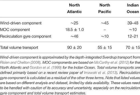
Table 1. Component of total WBC volume transports (Sv) in the North Atlantic, the North Pacific, and the Indian Ocean based on various previous studies.

The area of RR is determined subjectively. Although we examine the relation between RR and distribution area of STMW, it is difficult to define RR using hydrographic data. We cannot separate the “wind-driven Sverdrup circulation component” and inertial circulation component using hydrographic data (Wunsch and Roemmich, 1985; Hautala et al., 1994). Since we do not have a common criterion to define RR, RR is defined subjectively as a closed contour of dynamic height at 200 dbar relative to 1000 dbar. The depth of 200 dbar is a typical depth where STMW is located. Selected dynamic heights as a definition of RR are 137.5 (cm² s⁻²) for the North Pacific, 102.5 (cm² s⁻²) for the North Atlantic, 117.5 (cm² s⁻²) for the South Pacific, 100.0 (cm² s⁻²) for the South Atlantic and 120.0 (cm² s⁻²) for the Indian Ocean. The defined RR corresponds to previous descriptions of RR in each basin, in terms of its spatial coverage; the North Pacific for Suga and Hanawa (1995), the North Atlantic for Worthington (1976), the South Pacific for Ridgway and Dunn (2003), the South Atlantic for Peterson and Stramma (1991), and the Indian Ocean for Stramma and Lutjeharms (1997). We observe that defined RR area in the North Atlantic is the largest across the five basins.

Results

Common Definition of STMWs in the World Ocean

Before introducing a common criterion to define STMW, we first revisit fundamental oceanic structure associated with STMW and point out why we have different thresholds to define STMW in each basin. Because of the formation mechanism, STMW is characterized as a thermostad or a pycnostad (weakly stratified temperature layer or density layer) in summer temperature or density profiles. In dT/dz and PV profiles, STMW is characterized as dT/dz minimum layer or PV minimum layer, as summarized by Figure 5.4.1 in Hanawa and Talley (2001). dT/dz minimum layer or PV minimum layer are often used to define STMW along with temperature window or density window. The fundamental reason why we have different threshold of STMW is that temperature and density stratification is different from basin to basin (Figure 1). We need to adjust the temperature window and the dT/dz threshold values in order to define each STMW appropriately.

FIGURE 1

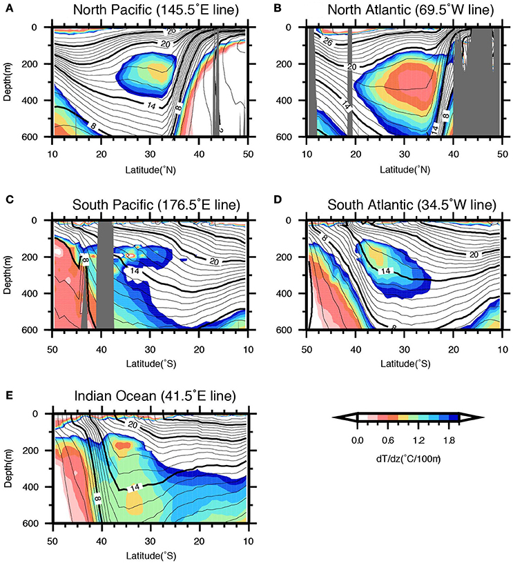
Figure 1. (A) Meridional temperature (°C; black contours) and vertical temperature gradient (dT/dz, °C/100 m; color shading) sections of the western part of the subtropical gyre in the North Pacific along 145.5°E line. (B–E) That of in the North Atlantic along 69.5°W line, South Pacific along 176.5°E line, South Atlantic along 34.5°W line, Indian Ocean along 41.5°E line, respectively. The hydrographic data is based on HydroBase version 2.0 dataset. Gray shade shows the bottom topography.

We first introduce a common definition of STMW using a single profile at 69.5°W and 32.5°N in the North Atlantic. Figure 2A shows dT/dz profile and NASTMW defined as a dT/dz minimum layer. NASTMW is defined as dT/dz < 1.0°C/100 m and temperature range of 16–22°C. The dT/dz threshold of 1.0°C/100 m defines upper boundary and lower boundary of NASTMW. Figure 2B shows a temperature profile at the same location and NASTMW defined by using core layer temperature (CLT). CLT is temperature at core layer. The position of core layer is identified as the minimum dT/dz within NASTMW (Figure 2A). Temperature window of CLT ± 1°C defines upper boundary and lower boundary of NASTMW in Figure 2B. The NASTMW defined by dT/dz criterion and CLT ± 1°C criterion matches well in this case. Figures 2C,D give another example in the North Pacific. Again, The NPSTMW defined by dT/dz criterion and CLT ± 1°C criterion matches well. We propose that any STMW could be defined with uniform criterion of CLT ± 1°C with a single temperature profile once we know CLT.

FIGURE 2

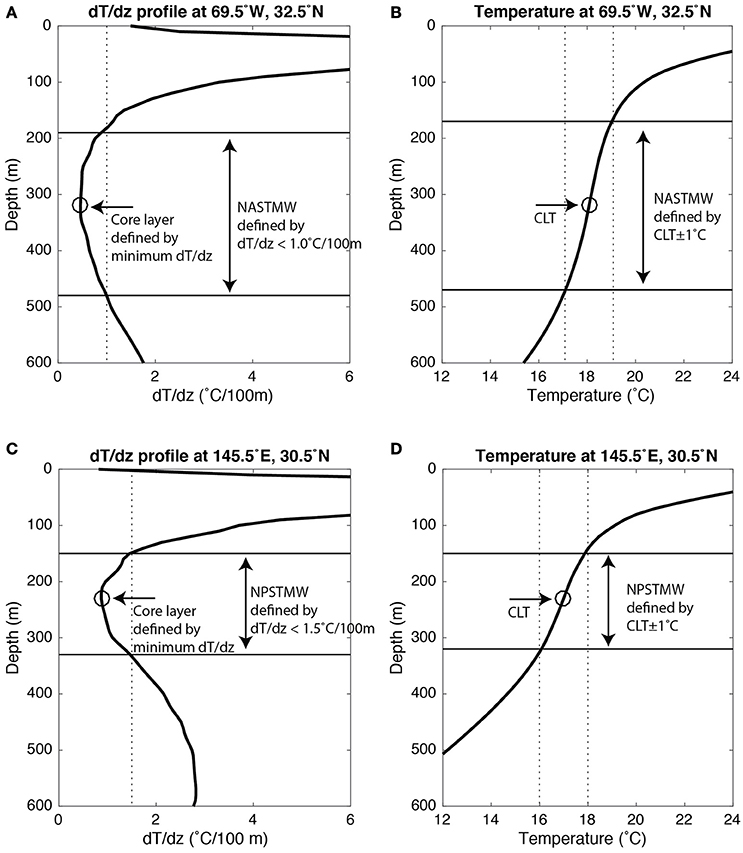
Figure 2. (A) dT/dz profile at 69.5°W and 32.5°N along with North Atlantic STMW (NASTMW) defined as dT/dz minimum layer. The vertical dotted line denotes 1.0°C/100 m dT/dz to be used to identify NASTMW. Black circle shows a position of core layer, defined as minimum dT/dz within the NASTMW. (B) Temperature profile at 69.5°W and 32.5°N. The vertical dotted line denotes core layer temperature (CLT)±1°C to identify NASTMW as a thermostad. Black circle shows CLT in the temperature profile. (C) Same as (A), but for the North Pacific STMW (NPSTMW) at 145.5°E and 30.5°N. (D) same as (B), but for the NPSTMW at 145.5°E and 30.5°N.

When it comes to define STMW using CLT for many temperature profiles, it is not practical to apply different CLTs at each temperature profiles to extract STMW. We calculate averaged CLT for each STMW by averaging over individual CLTs. As such, an overview of (our approach) defining STMWs with temperature profiles follows. Firstly, different criteria of temperature window and dT/dz threshold are applied to extract CLTs at every profile. Secondly, the extracted individual CLTs are averaged to calculate averaged CLT for each STMW. Thirdly, we define STMW as a thermostad applying a condition of averaged CLT ± 1°C with its layer thickness >100 m.

The first step is to extract core layer water properties at each grid point in each STMW. Each STMW in five different basins are defined by applying different criteria of temperature window and dT/dz thresholds. For the case of NASTMW, it is 16–22°C for temperature and 1.0°C/100 m for dT/dz followed by Kwon and Riser (2004). For the case of NPSTMW, it is 14–20°C for temperature and 1.5°C/100 m for dT/dz followed by Suga and Hanawa (1995). All different criteria in different basins are summarized in Table 2. Followed by Tsubouchi et al. (2010), the threshold of dT/dz is changed continuously from 2.0 to 0.0°C/100 m with 0.01°C/100 m interval in order to extract Indian Ocean STMW (IOSTMW). We further apply thickness threshold of STMW (thicker than 30 m) and distribution area criteria. This thickness and distribution area criteria eliminate thin dT/dz minimum layer or dT/dz minimum layer located outside of western part of the subtropical gyre. The extracted STMWs in each basin are shown in colored dots both on the geographical plane and TS plane in Figure 3. The dT/dz minimum layer that is extracted with different criteria of temperature window and dT/dz threshold, but eliminated by thickness or distribution area criteria is shown in gray in the geographical plane and the TS plane.

TABLE 2

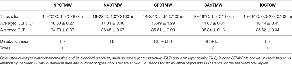
Table 2. Criteria of temperature and dT/dz thresholds used to extract STMWs in each basin and their relation to flow field.

FIGURE 3

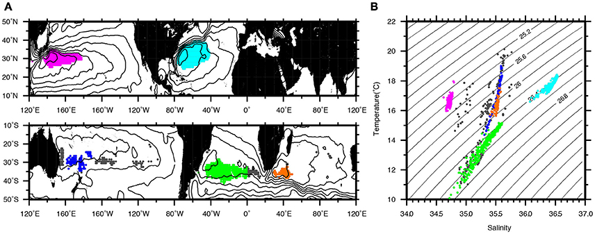
Figure 3. (A) Distribution area of STMWs extracted using different criteria of temperature window and dT/dz threshold in each basin. Colored dots show defined STMWs and gray dots show the excluded dT/dz minimum layer by the thickness or distribution area conditions. See the main text for detail. Contours show the dynamic height (cm² s⁻²) at 200 m relative to 1000 m. Contour interval is 10.0 (cm² s⁻²). (B) CLT and core layer salinity (CLS) of the extracted STMWs in each basin on the T-S plane. Colored dots show CLT and CLS associated with the extracted STMWs in each basin and gray dots show that associated with the excluded dT/dz minimum layer.

The second step is to calculate averaged core layer water properties for each STMW. The individual core layer water properties shown in Figure 3B on TS plane are averaged over each STMW to calculate averaged CLT and averaged core layer salinity (CLS) for each STMW. Obtained averaged CLT and averaged CLS are summarized in Table 2. We should note that these values represent hemisphere summer period and centered around year of 1990's. Moreover, amount of data to be reconstructed the Hydrobase dataset differs from basin to basin. Obtained mean core layer water characteristics of NPSTMW, NASTMW, IOSTMW are consistent with previous studies: Masuzawa (1969) and Suga and Hanawa (1995) for NPSTMW; Worthington (1959) and Kwon and Riser (2004) for NASTMW; Tsubouchi et al. (2010) for IOSTMW, respectively. The wide CLT range of South Pacific STMW (SPSTMW; 14.5–19.0°C in Figure 3B) covers the water characteristics of three types of SPSTMW (Tsubouchi et al., 2007). The wide water property range of South Atlantic STMW (SASTMW; 11.0–15.0°C for CLT and 34.9–35.6 for CLS) in Figure 3B covers the water characteristics of type 2 and type 3 SASTMW (Provost et al., 1999; Sato and Polito, 2014). Different types of SPSTMW and SASTMW are not resolved in the HydroBase. Rather, they are represented as STMW with wide water property range. The water characteristics of type 1 SASTMW (26.2σ_θ and 17.0 ± 1.0°C) are not extracted using HydroBase dataset. Since type 1 SASTMW is thinner than that of type 2 and type 3 (Provost et al., 1999; Sato and Polito, 2014), HydroBase may not be able to capture the signal of type 1 SASTMW.

The third step is to define STMW as a thermostad. Based on the averaged CLT of each STMW calculated above, STMW is defined as a thermostad (a layer weakly stratified in temperature) applying a criterion of averaged CLT ± 1°C with its layer thickness greater than 100 m. This threshold is equivalent to dT/dz < 2°C/100 m, assuming a monotonic temperature stratification. Furthermore, the conditions of the STMW distribution area are applied to the North Atlantic (west side of 30°W) and to the South Atlantic (west side of 0°) in order to exclude Madeira Mode Water (Siedler et al., 1987) and South Atlantic Eastern STMW (Provost et al., 1999). They are located in the eastern part of the subtropical gyre, having almost the same temperature as STMW.

Finally, we note the choice of temperature window of averaged CLT ± 1°C. This temperature window is arbitratory on principal, but it has some limit in order to extract different STMWs with same condition across the five basins. Temperature window should be limited between averaged CLT ± 0.8°C and averaged CLT ± 1.2°C. Assuming monotonic temperature stratification, temperature window of ±0.8 and ±1.2°C are equivalent to dT/dz < 1.6°C/100 m and dT/dz < 2.4°C/100 m, respectively. Temperature window of ±0.8°C is the lower limit to extract SPSTMW appropriately, and temperature window of ±1.2°C is the upper limit to extract NASTMW appropriately (Figure 1).

Horizontal Structure of STMW in the World Ocean

Figure 4 shows the distribution of STMW thickness defined by the common criterion. The defined STMW captures the typical STMW spatial structure. The defined STMWs are located in the western part of the subtropical gyre in each basin and the thickness of each STMW qualitatively reflects STMW thickness shown in meridional temperature section (Figure 1). NASTWM has the greatest thickness of 276 ± 23 (m) with the largest horizontal distribution area. NPSTMW and IOSTMW have similar thickness (168 ± 16 and 155 ± 16 m, respectively), but NPSTMW has the larger horizontal distribution area. As already described by the previous studies (Masuzawa, 1969; Suga and Hanawa, 1995 for NPSTMW; Worthington, 1959; Kwon and Riser, 2004 for NASTMW; Tsubouchi et al., 2010 for IOSTMW, respectively), major portions, including the thickest part, of NASTMW, NPSTMW, and IOSTMW are located within RR in each basin. Previous studies also suggest that SPSTMW and SASTMW can be categorized into three distinct types of STMW, and some of them are located in the eastward flow region (Tsubouchi et al., 2007 for SPSTMW; Provost et al., 1999; Sato and Polito, 2014 for SASTMW). As reported by Provost et al. (1999) and Sato and Polito (2014), thicker SASTMW (>150 m) is located in the eastward flow region of 32–37°S and 40–20°W. We note that a part of SPSTMW (west type of STMW, Tsubouchi et al., 2007) cannot be extracted with the newly proposed criterion of averaged CLT ± 1°C due to the wider core layer water property range of SPSTMW. The west type of SPSTMW has CLT of ~19.2°C (Tsubouchi et al., 2007), which is significantly higher than the SPSTMW averaged CLT of 16.94 ± 1.29°C (Table 2).

FIGURE 4

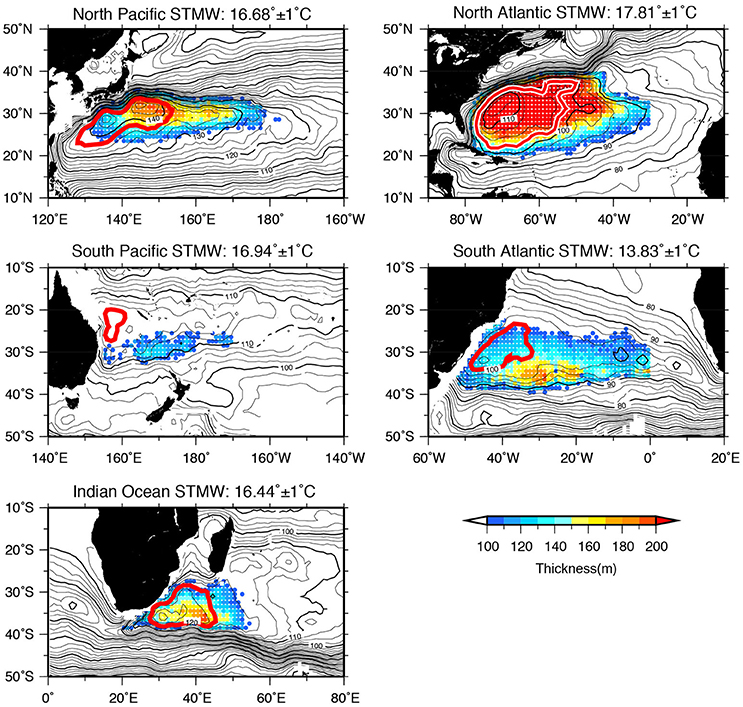
Figure 4. Spatial distribution of STMW thickness (m) in the world ocean. STMWs in each basin are defined by the newly proposed common definition of averaged CLT ± 1 °C with its layer thickness greater than 100 m. Averaged CLT for each STMW is shown at top of each plot. The red closed contour represents RR subjectively determined in this study. Background contour shows the dynamic height (cm² s⁻²) at 200 m relative to 1000 m. Contour interval is 2.5 (cm² s⁻²) for thin lines and 10.0 (cm² s⁻²) for bold lines.

Gathering previous finding about the STMW distribution area and number of types belonging to STMW in each basin, we can categorize the STMW into two groups as shown in Table 2. The first group of STMWs (NPSTMW, NASTMW, and IOSTMW) has a single water characteristic and it is largely located within RR. The second group of STMWs (SPSTMW and SASTMW) has multiple types of water and it is located inside RR and in the eastward flow region.

It is reasonable that STMW formed within RR tends to have uniform water property. Since the streamlines are generally closed in RR, RR prepares the field with almost the same water property. It is also reasonable that STMW formed outside RR tends to have different water properties from that formed within RR because a density front in the wintertime mixed layer exists between the area inside RR and the area outside RR.

Vertical Structure of STMWs in the World Ocean

Figure 5 shows the histograms of dT/dz, dS/dz, and PV of STMW in the world ocean to illustrate the similarities and dissimilarities of the vertical structure of STMWs across the different basins. Histogram is made based on each volume element within the defined mode water. The number of 3D-grid points in each STMW are also shown to indicate the volume of STMW. NASTMW has the lowest dT/dz (1.05 ± 0.40°C/100 m), PV (114 ± 50 × 10⁻¹² m⁻¹s⁻¹) and largest grid number, showing that NASTMW is the largest STMW with the most homogeneous vertical structure of temperature and density in the world ocean. NPSTMW and IOSTMW have similar shapes of dT/dz, dS/dz, and PV. This suggests that the vertical structures of temperature, salinity and density of NPSTMW and IOSTMW are almost the same. However, volume of NPSTMW is 1.8 times larger than that of IOSTMW. Looking at the thickness distribution of NPSTMW and IOSTMW in Figure 4, the volume difference mainly comes from the size of the horizontal distribution area. SPSTMW shows the highest dT/dz (1.87 ± 0.30°C/100 m) and PV (245 ± 43 × 10⁻¹² m⁻¹s⁻¹), showing that SPSTMW has the least homogeneous vertical structure of temperature and density in the world ocean.

FIGURE 5

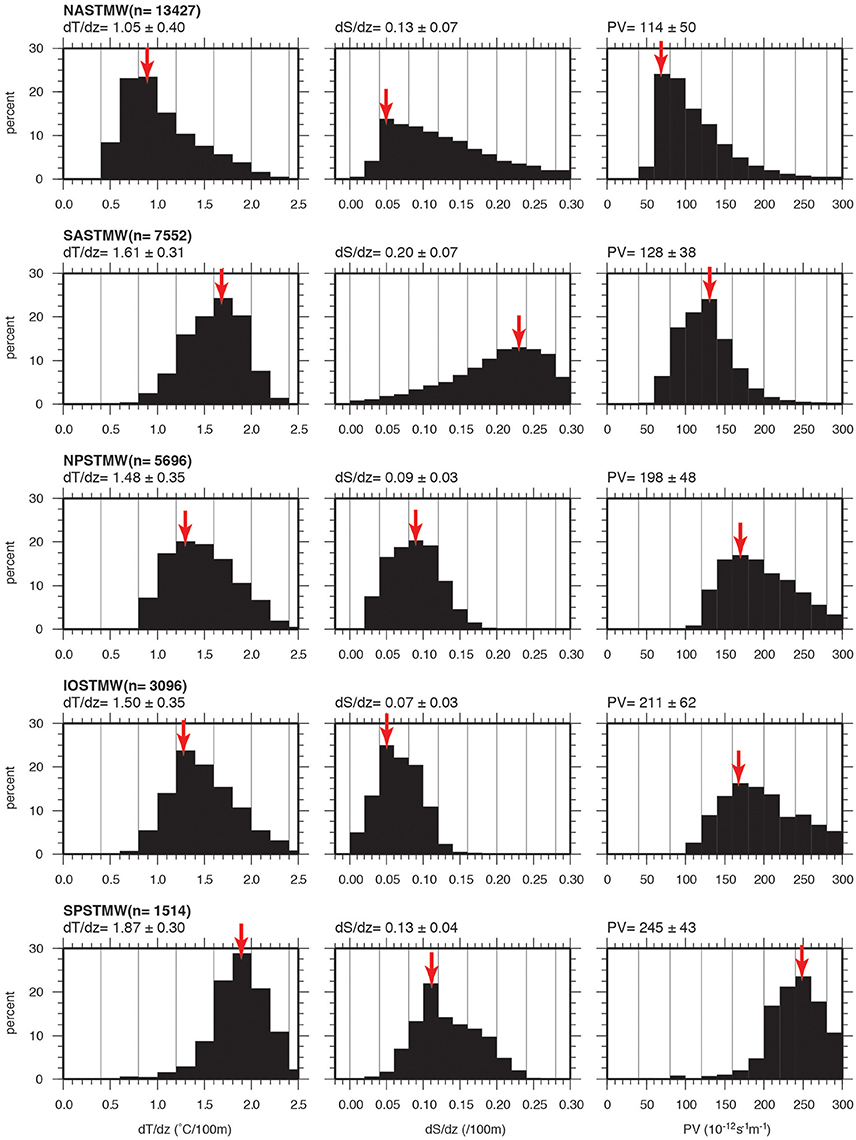
Figure 5. Histogram of dT/dz (°C/100 m), dS/dz (/100 m), and PV (10⁻¹² m⁻¹s⁻¹) belonging to each STMW. Histogram is made based on each volume element within the defined mode water. Red arrow indicates the mode value of each property. Number of 3D-grids in each STMW, mean and standard deviation of each property are also shown on top of each panel.

It is notable that some histograms are deviated from the normal distribution. The dT/dz, dS/dz, and PV histograms of NASTMW have positive skewness of 1.00, 0.97, 1.84, respectively. The dS/dz histogram of SASTMW has negative skewness of −0.53. For the NASTMW, it is due to the uniform STMW definition. Because of the common definition of averaged CLT ± 1°C with its thickness >100 m, it defines all thermostads which has temperature stratification of <2.0°C/100 m (assuming that temperature stratification is constant in depth). This results in a long tail toward 2.0°C/100 m in dT/dz histogram of NASTMW. This also affects on dS/dz and PV histograms of NASTMW. The negative skewness of SASTMW dS/dz histogram is due to higher salinity stratification in lower part of SASTMW as discussed in next paragraph.

The vertical structure of SASTMW is significantly different from the other STMWs. Figure 6 shows meridional sections of dT/dz, dS/dz, and PV in the North Pacific (along 145.5°E line) and the South Atlantic (along 34.5°W line). While meridional sections of dT/dz in the North Pacific and the South Atlantic contain distinctive dT/dz minimum layer corresponding to NPSTMW and SASTMW, respectively, the distributions of dS/dz are significantly different from each other. In the North Pacific, weak temperature stratification (<1.4°C/100 m) corresponds to weak salinity stratification (<0.1/100 m), indicating that NPSTMW is a remnant of the winter mixed layer. On the other hand, in the South Atlantic, weak temperature stratification (<1.4°C/100 m) contains not only weak salinity stratification (<0.1/100 m) in the upper part but also higher salinity stratification (>0.1/100 m) in the lower part. The layer of this higher salinity stratification implies that this layer is not the remnant of the winter mixed layer, but rather another formation mechanism may exist. Because of this higher salinity stratification, SASTMW has lower PV (<128 ± 38 × 10⁻¹² m⁻¹s⁻¹) than that of NPSTMW (<198 ± 48 × 10⁻¹² m⁻¹s⁻¹). The vertical structure of SASTMW is characterized by highly density-compensating T/S stratification. A possible mechanism to form this layer (SASTMW) will be discussed in the Discussion Section.

FIGURE 6

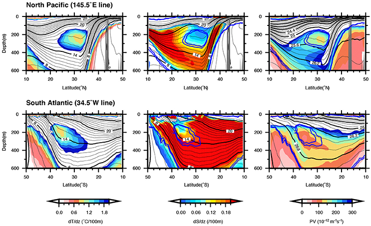
Figure 6. (Top panels) Meridional section of dT/dz (°C/100 m), dS/dz (/100 m), and PV (10⁻¹² m⁻¹s⁻¹) in the North Pacific along the 145.5°E line. (Bottom panels) same as top panels, but in the South Atlantic along the 34.5°W line. The blue contours in the dS/dz section and the PV section denote the 1.4 and 1.6 °C/100 m contours.

Figure 7 summarizes the characteristics of vertical structure of each STMW using the mode values of dT/dz, dS/dz, and PV. Because of the positive skewness of NASTMW histogram, mode value captures its major vertical structure of NASTWM better than mean values. It is shown that NASTMW has the strongest vertical homogeneity in temperature, salinity, and density. NPSTMW and IOSTMW have moderate vertical homogeneity in temperature and density. The vertical salinity stratification of IOSTMW is as low as that of NASTMW. This may be due to the smaller volume size of IOSTMW and weaker background stratification in the region. SPSTMW has the weakest vertical homogeneity in temperature and density. SASTMW has unique vertical structure sustaining second lowest PV mode value with density-gradient-compensating high dT/dz and high dS/dz. Finally, we note that most of the above conclusion also holds if we use mean value instead of mode values of the histogram. The only significant difference is that dS/dz mean value of NASTMW (0.13 ± 0.07 /100 m) is larger than that of NPSTMW (0.09 ± 0.03 /100 m) and IOSTMW (0.07 ± 0.03 /100 m) due to the positive skewness of dS/dz histogram.

FIGURE 7

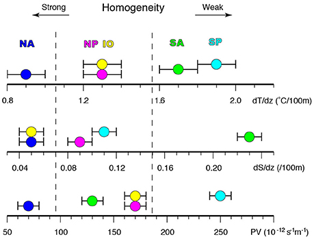
Figure 7. The mode value of dT/dz (°C/100 m; top coordinate), dS/dz (/100 m; middle coordinate), and PV (10⁻¹² m⁻¹s⁻¹; bottom coordinate) belonging to each STMW. Error bar shows the width of histogram bar in Figure 5. NA, NP, SA, SP, and IO correspond to NASTMW, NPSTMW, SASTMW, SPSTMW, and IOSTMW, respectively.

Major Factors to Influence the STMW Thickness in the World Ocean

It is generally recognized that thicker STMWs are located in the Northern Hemisphere with stronger WBC and stronger winter cooling. Here, we consider which factor is more important to form thicker STMW by comparing STMWs among basins. Figure 8 shows a scatter plot of STMW thickness against other quantities, such as surface heat flux, typical WBC transports and MTD. Figure 8A shows that larger surface heat flux does not appear necessary to result in thicker STMW. In spite of the strongest winter cooling in its formation area, NPSTMW is much thinner than NASTMW and comparable to IOSTMW, which is exposed to much weaker cooling. Figure 8B shows a weak positive relationship between WBC transport and thickness of STMW. The North Atlantic hosts the strongest WBC and thickest STMW in the world ocean. While the Indian Ocean WBC is slightly larger than that in the North Pacific, these basins have almost the same STMW thickness. The South Pacific hosts the thinnest and the weakest WBC. The South Atlantic may not have to follow this liner relationship because SASTMW has the density-compensating T/S vertical stratification (Figure 6). The weak positive relationship between the WBC transport and the STMW thickness is supported by tight positive relationship between the STMW thickness and MTD (Figure 8C). This result suggests that thicker STMW tends to be accompanied with stronger WBC transport. Although, winter cooling is essential to form STMW itself, the difference in STMW thickness between basins may not necessary due to the difference in strength of winter cooling.

FIGURE 8

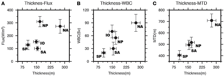
Figure 8. Scatter plot of STMW thickness (m) against other background quantities: (A) STMW thickness and surface heat flux (Wm⁻²), (B) STMW thickness and WBC transport (Sv), and (C) STMW thickness and MTD (m). Error bar of STMW thickness, surface heat flux, and MTD show standard deviation of quantified quantities with different size of averaging window. Error bar of WBC shows defined uncertainties in this study. NA, NP, SA, SP, and IO correspond to NASTMW, NPSTMW, SASTMW, SPSTMW, and IOSTMW, respectively.

It needs to be clarified that this comparison analysis has a fundamental limitation that restricts the robustness of conclusion. That is, we have only five realizations of STMWs in the world ocean. On the other hand, STMW thickness is a result of many different processes. The strength of upper ocean stratification at the beginning of cooling season, evaporation and precipitation, and the intrusion of higher stratified water from north of WBC all influence the development of winter mixed layer. The diffusivity and mixing rate from the formation region and the distribution region may differ between different basins. All of these effects could offset or distort the relationship between STMW thickness and strength of winter cooling or STMW thickness and strength of WBC. This means that we would never come up with a statistically robust conclusion on which factor primary influences on the STMW thickness. Nevertheless, it is still interesting to relate STMW thickness against these back ground forcing conditions in five different basins as this provides an indication that strength of WBC has better relationship than strength of winter cooling has.

Discussion

Why the North Atlantic Hosts the Thickest STMW in the World Ocean?

In this section, we discuss why the North Atlantic hosts the thickest STMW in the world ocean from a vorticity dynamics point of view. In the wind-driven general circulation model, the recirculation gyre appears as a strong sub-basin scale inertial flow with homogeneous PV. Cessi et al. (1987) examines how the recirculation gyre appears using a simple barotropic model driven by anomalously low PV applied at the northern boundary of a rectangular ocean. This boundary forcing mimics the effect of adiabatic or diabatic forcing producing low PV at the poleward edge of a subtropical gyre. They show that homogeneity of PV increases and the size and strength of the recirculation gyre increases when anomalously low PV at the northern boundary is intensified. Although, they clearly show how the recirculation gyre responds to changes in low PV input, it is still unclear what is the source of low PV at the poleward edge of the subtropical gyre.

We argue that both thicker STMW and stronger recirculation gyres are fundamentally based on the same ocean structure, such as a deeper main thermocline and corresponding steeper slope of the main thermocline in the western part of the subtropical gyre. Based on this argument, we assume that the strength of the recirculation gyre is proportional to STMW PV, calculated using Equation (1). This assumption seems to work well qualitatively when we compare observed strength of the recirculation gyre and PV of STMW. The strength of the recirculation gyre in the North Atlantic (~46 Sv) is stronger than that in the North Pacific (10–15 Sv) and in the Indian Ocean (12–20 Sv). The PV of NASTMW (114 ± 50 × 10⁻¹² m⁻¹s⁻¹) is lower than the PV of NPSTMW (198 ± 48 × 10⁻¹² m⁻¹s⁻¹) and the PV of IOSTMW (211 ± 62 × 10⁻¹² m⁻¹s⁻¹).

Combining the result of Cessi et al. (1987) and our “comparison study of STMW,” two implications can be drawn under the assumption that the strength of the recirculation gyre is proportional to STMW PV. First implication is that the thickness of STMW is determined by the input of low PV at the edge of the subtropical gyre. STMW thickness appears correlated to the PV of STMW because STMW PV and STMW dT/dz are generally correlated except for SASTMW (Figure 7). Second implication is that the low PV carried by the WBC is the dominant factor to maintain input of low PV at the poleward edge of the subtropical gyre. The implication that the strength of winter cooling may not strongly influence the thickness of STMW means that the strength of winter cooling may not play a key role in producing low PV at the poleward boundary of the subtropical gyre. This implication gives a physical interpretation to the low PV applied at the northern boundary of a rectangular ocean by Cessi et al. (1987).

Regarding the input of low PV carried by the WBC at the poleward edge of the subtropical gyre where STMW is formed (north-western part for North Pacific and North Atlantic; south-western part for Indian Ocean), only the through flow component of the WBC (i.e., “wind-driven” component and MOC component) should be considered. The inertial recirculation gyre does not bring any low PV from lower latitude into the region. Assuming that the input of low PV carried by the WBC is proportional to the volume transport of the “wind-driven” component and MOC component in each basin, the North Atlantic (~44 Sv), the North Pacific (~45 Sv), and the Indian Ocean (49–58 Sv) have almost the same magnitude of gross input of low PV (Table 1). Here, we argue that the North Atlantic has the ideal condition to host the largest net input of low PV compared to the other basins. That is, it has no effective mechanism allowing anomalous low PV to escape from the gyre or dissipate within the gyre. The Indian Ocean intermittently releases Agulhas eddies bringing out low PV into the South Atlantic (Goni et al., 1997). These eddies effectively transfer low PV from the Indian Ocean to the South Atlantic. In the North Pacific, the complex bottom topography such as Tokara strait and Izu-Ogasawara ridge may dissipate low PV carried by the Kuroshio effectively. The Tsushima Current may also transfer low PV from the North Pacific to the Sea of Japan continuously. On the other hand, the equilibrium of PV budget in the North Atlantic may be achieved as a combination of relatively smaller PV dissipation coefficient and higher PV contrast between inside and outside of recirculation gyre. We conclude that the North Atlantic is the basin to host the largest net input of low PV to cause the thickest STMW and the strongest recirculation, yielding the strongest WBC in the world ocean.

Finally, we should mention there are other processes which play a role in PV budget in this region. In particular, the role of eddy and frontal processes in the STMW formation region may be important. It is likely that mesoscale eddy plays a role on modulating air-sea interaction by promoting convection. This would create anomalous low PV (Cerovecki and Marshall, 2008). Horizontal and vertical velocity shear near the frontal region can become important in Ertel PV (Joyce et al., 2009). Abrupt wind at frontal region could extract/inject PV in the frontal region (Thomas and Lee, 2005; Thomas and Joyce, 2010; Thomas et al., 2013). Quantifications of these components in the PV budget are necessary to come up with robust view on why the North Atlantic hosts the thickest STMW and stronger recirculation gyre in the world ocean.

Possible Formation Mechanisms of SASTMW

The uniqueness of the vertical structure of SASTMW is highlighted by comparing it against the other STMWs. The SASTMW vertical structure is characterized by a highly density-compensating T/S stratification (Figure 6). We point out that the thick part of SASTMW (>150 m) is located outside the RR (Provost et al., 1999; Sato and Polito, 2014). Moreover, the horizontal Turner angle at the sea surface in the likely formation region for SASTMW (60–30°W, 30–50°S) is higher than in the likely formation regions of the other STMWs (Johnson, 2006). We speculate that formation mechanism of SASTMW may be similar to that of North Pacific Eastern Subtropical Mode Water (NPESTMW; Hautala and Roemmich, 1998) and South Pacific Eastern STMW (SPESTMW; Wong and Johnson, 2003). NPESTMW and SPESTMW are located outside the RR and their vertical structures are characterized by a density-compensating T/S stratification (Toyama and Suga, 2010). Hosoda et al. (2001) suggests that vertical structure of low PV associated with NPESTMW is primarily formed by widely spaced density outcrop lines in its formation region. The different types of SASTMW may have similar density but quite distinct temperature and salinity, forming a highly density-compensating T/S vertical structure. Examination of this hypothesis is out of the scope of the present study and further study is required.

Summary and Conclusion

This paper proposes a new approach to quantify and compare spatial structure of STMWs in the world ocean by offering a common criterion of STMWs. STMW is defined as a thermostad (a layer weakly stratified in temperature) applying a criterion of averaged CLT ± 1°C with its layer thickness greater than 100 m. This condition is equivalent to dT/dz < 2°C/100 m assuming homogeneous temperature stratification. In order to calculate the averaged CLT, individual CLTs need to be identified for each temperature profiles in advance. Averaged CLT is then calculated by averaging over individual CLTs within associated STMW. Temperature windows of ±1°C can be varied between ±0.8 and ±1.2°C.

The horizontal and vertical structure of STMW defined with the common criterion matches well to previous studies. Regarding the characteristics of horizontal structure, we see features reported by previous studies individually. That is, NASTMW, NPSTMW, and IOSTMW have a single type of water characteristics and are located almost within the RR. On the other hand, SPSTMW and SASTMW have multi-types of water characteristics and are located both in the RR and the eastward flow region. We suggest that STMWs can be categorized into two groups as above. Regarding the characteristics of vertical structure, NASTMW has the most homogeneous vertical structure in temperature, salinity and density. NASTWM is the thickest (276 ± 23 m) and volumetrically largest STMW in the world ocean. NPSTMW and IOSTMW have similar vertical structure in temperature, salinity, and density. Although they have almost same thickness (168 ± 16 and 155 ± 16 m, respectively), the volume of NPSTMW is 1.8 times larger than that of IOSTMW. SASTMW has an unique vertical structure, highlighted by density compensating T/S stratification. SPSTMW is the thinnest STMW (108 ± 8 m) and volumetrically smallest STMW in the world ocean.

The major factors that influence the STMW thickness is investigated by comparing quantified STMW thicknesses against the strength of winter cooling and typical WBC volume transports. Although, we cannot obtain a simple relationship due to the complex STMW formation mechanisms and uncertainty associated with WBC volume transports, we find an indication that thicker STMWs tend to be accompanied with stronger WBC. The strength of winter cooling may not play a major role in determining the STMW thickness in each basin. In spite of the strongest winter cooling in its formation area, NPSTMW is much thinner than NASTMW and comparable to IOSTMW, which is exposed to much weaker cooling.

The schematic in Figure 9 summarizes this study, and provides a working hypothesis for further STMW studies. The North Atlantic hosts the thickest and the largest STMW and the strongest recirculation gyre in the world ocean. The North Atlantic may effectively preserve low PV carried by the Gulf Stream. The North Pacific and Indian Oceans have STMWs with moderate thickness. In terms of volume of STMW, the North Pacific (the Indian Ocean) hosts 42% (23%) volume of NASTMW. Although, the WBCs (the Kuroshio and the Agulhas Current) may carry low PV to the western part of subtropical gyre as much as the Gulf Stream does, processes to dissipate low PV may exist in these two basins. The South Pacific has the thinnest STMW. SPSTMW has three-types of STMW located both in the RR and the eastward flow region. The South Atlantic has a unique STMW which is mainly distributed outside the RR with highly density-compensating T/S stratification. The different types of SASTMW with similar density might overlap each other and form low density stratification.

FIGURE 9

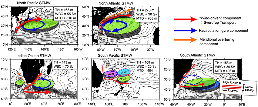
Figure 9. Schematic figure to illustrate relationship between components of WBC and types of STMW in each basin. WBC is consists of “wind-driven” component (red arrow), recirculation gyre component (blue arrow) and meridional overturning component (orange arrow), and number of types of STMW are shown by colored columns. The averaged value of STMW thickness (m; TH), WBC total volume transport (Sv), and MTD (m) are also shown. Contour shows the dynamic height (cm² s⁻²) at 200 m relative to 1000 m. Contour interval is 2.5 (cm² s⁻²) for thin lines and 10.0 (cm² s⁻²) for bold lines.

Highlighting the similarities and dissimilarities of STMWs in different basins provides insight into the relative dominance of formation mechanisms. We would like to see future STMW studies focus on two aspects: firstly, a comparison study of STMWs and secondly a detailed study of individual STMW. These subsequent studies on STMWs will provide better understanding of mid-latitude WBC systems where there are complex interactions between dynamics and thermodynamics and between ocean and atmosphere.

Author Contributions

TT conducted the data analysis, with regular input from TS and KH. TT wrote the manuscript with support by TS.

Conflict of Interest Statement

The authors declare that the research was conducted in the absence of any commercial or financial relationships that could be construed as a potential conflict of interest.

The reviewer GR and handling Editor declared their shared affiliation, and the handling Editor states that the process nevertheless met the standards of a fair and objective review.

Acknowledgments

We acknowledge fruitful discussions with members of Physical Oceanography Group at Tohoku University. This study was performed as a part of the twenty-first Century Center-Of-Excellence (COE) Program “Advanced Science and Technology Center for Dynamic Earth (E-ASTEC)” at Tohoku University. Comments from two reviewers improved the quality of paper. Dr Jeremy Grist did English editing. The second author (TS) was supported by the Grant-in-Aid from the Japan Society for the Promotion of Science (15H02129 and 25287118).

Supplementary Material

The Supplementary Material for this article can be found online at: https://www.frontiersin.org/article/10.3389/fmars.2016.00270/full#supplementary-material

References

Akima, H. (1970). A new method of interpolation and smooth curve fitting based on local procedures. J. Assoc. Comput. Math. 17, 589–602. doi: 10.1145/321607.321609

CrossRef Full Text | Google Scholar

Alexander, M. A., Deser, C., and Timlin, M. S. (1999). The reemergence of SST anomalies in the North Pacific Ocean. J. Clim. 12, 2419–2433. doi: 10.1175/1520-0442(1999)012<2419:TROSAI>2.0.CO;2

CrossRef Full Text | Google Scholar

Bryden, H. L., Beal, L. M., and Duncan, L. M. (2005). Structure and transport of the agulhas current and its temporal variability. J. Oceanogr. 61, 479–492. doi: 10.1007/s10872-005-0057-8

CrossRef Full Text | Google Scholar

Cassou, C., Deser, C., and Alexander, A. M. (2007). Investigating the impact of reemerging sea surface temperature anomalies on the winter atmospheric circulation over the North Atlantic. J. Clim. 20, 3510–3526. doi: 10.1175/JCLI4202.1

CrossRef Full Text | Google Scholar

Cerovecki, I., and Marshall, J. (2008). Eddy modulation of air–sea interaction and convection. J. Phys. Oceanogr. 38, 65–83. doi: 10.1175/2007JPO3545.1

CrossRef Full Text | Google Scholar

Cessi, P., Ierley, G., and Young, W. (1987). A model of the inertial recirculation driven by potential vorticity anomalies. J. Phys. Oceanogr. 17, 1640–1652. doi: 10.1175/1520-0485(1987)017<1640:AMOTIR>2.0.CO;2

CrossRef Full Text | Google Scholar

de Boyer Montégut, C., Madec, G., Fischer, A., Lazar, A., and Iludicone, D. (2004). Mixed layer depth over the global ocean: an examination of profile data and a profile-based climatology. J. Geophys. Res. 109:C12003. doi: 10.1029/2004jc002378

CrossRef Full Text | Google Scholar

Dewar, W. K., Samelson, R. M., and Vallis, G. K. (2005). The ventilated pool: a model of subtropical mode water. J. Phys. Oceanogr. 35, 137–150. doi: 10.1175/JPO-2681.1

CrossRef Full Text | Google Scholar

Drijfhout, S. S., Marshall, D. P., and Dijkstra, H. A. (2013). “Conceptual models of the wind-driven and thermohaline circulation,” in Ocean Circulation and Climate - A 21st Century Perspective, 2nd Edn, eds G. Siedler, S. M. Griffies, W. J. Gould, and J. Church (London: Academic Press), 257–282.

Goni, G. J., Garzoli, S. L., Roubicek, A. J., Olson, D. B., and Brown, O. B. (1997). Agulhas ring dynamics from TOPEX/POSEIDON satellite altimeter data. J. Mar. Res. 55, 861–883. doi: 10.1357/0022240973224175

CrossRef Full Text | Google Scholar

Gordon, A. L., Susanto, R. D., and Ffield, A. (1999). Throughflow within makassar strait. Geophys. Res. Lett. 26, 3325–3328. doi: 10.1029/1999GL002340

CrossRef Full Text | Google Scholar

Hanawa, K., and Talley, L. D. (2001). “Mode waters,” in Ocean Circulation and Climate: Observing and Modelling the Global Ocean, eds G. Siedler, J. Church, and J. Gould (London: Academic Press), 373–386.

Hautala, S. L., and Roemmich, D. H. (1998). Subtropical mode water in the Northeast Pacific Basin. J. Geophys. Res. 103, 13055–13066.

Google Scholar

Hautala, S. L., Roemmich, D. H., and Schmitz, W. J. (1994). Is the North Pacific in sverdrup balance along 24-degrees-n. J. Geophys. Res. 99, 16041–16052.

Google Scholar

Holte, J., and Talley, L. (2009). A new algorithm for finding mixed layer depths with applications to argo data and subantarctic mode water formation. J. Atmos. Oceanic Technol. 26, 1920–1939. doi: 10.1175/2009jtecho543.1

CrossRef Full Text | Google Scholar

Hosoda, S., Xie, S. P., Takeuchi, K., and Nonaka, M. (2001). Eastern North pacific subtropical mode water in a general circulation model: formation mechanism and salinity effects. J. Geophys. Res. 106, 19671–19681. doi: 10.1029/2000JC000443

CrossRef Full Text | Google Scholar

Huang, R. X., and Russell, S. (1994). Ventilation of the subtropical North Pacific. J. Phys. Oceanogr. 24, 2589–2605.

Google Scholar

Imawaki, S., Bower, A., Beal, L. M., and Qiu, B. (2013). “Western boundary currents,” in Ocean Circulation and Climate - A 21st Century Perspective, 2nd Edn, eds G. Siedler, S. M. Griffies, W. J. Gould, and J. Church (London: Academic Press), 305–338.

Johnson, G.C. (2006). Generation and initial evolution of a mode water theta-S anomaly. J. Phys. Oceanogr. 36, 739–751. doi: 10.1029/2008gl035918

CrossRef Full Text | Google Scholar

Josey, S. A., Kent, E. C., and Taylor, P. K. (1998). The Southampton Oceanography Centre (SOC) Ocean - Atmosphere Heat, Momentum and Freshwater Flux Atlas. Southampton Oceanography Centre Report.

Joyce, T. M., Thomas, L. N., and Bahr, F. (2009). Wintertime observations of subtropical mode water formation within the Gulf stream. Geophys. Res. Lett. 36:L02607. doi: 10.1029/2008GL035918

CrossRef Full Text | Google Scholar

Kelly, K. A., Small, R. J., Samelson, R. M., Qiu, B., Joyce, T. M., Kwon, Y.-O., et al. (2010). Western boundary currents and frontal air–sea interaction: gulf stream and kuroshio extension. J. Clim. 23, 5644–5667. doi: 10.1175/2010JCLI3346.1

CrossRef Full Text | Google Scholar

Kobashi, F., and Kubokawa, A. (2011). Review on north pacific subtropical countercurrents and subtropical fronts: role of mode waters in ocean circulation and climate. J. Oceanogr. 68, 21–43. doi: 10.1007/978-4-431-54162-2_2

CrossRef Full Text | Google Scholar

Kobayashi, T., and Suga, T. (2006). The indian ocean hydrobase: a high-quality climatological dataset for the Indian Ocean. Prog. Oceanogr. 68, 75–114. doi: 10.1016/0079-6611(95)00013-5

CrossRef Full Text | Google Scholar

Kwon, Y.-O., Alexander, M. A., Bond, N. A., Frankignoul, C., Nakamura, H., Qiu, B., et al. (2010). Role of the gulf stream and Kuroshio–Oyashio systems in large-scale atmosphere–ocean interaction: a review. J. Clim. 23, 3249–3281. doi: 10.1175/2010JCLI3343.1

CrossRef Full Text | Google Scholar

Kwon, Y. O., and Riser, S. C. (2004). North atlantic subtropical mode water: a history of ocean-atmosphere interaction 1961–2000. Geophys. Res. Lett. 31:L19307. doi: 10.1029/2004GL021116

CrossRef Full Text | Google Scholar

Lozier, M. S., Owens, W. B., and Curry, R. G. (1995). The climatology of the North Atlantic. Prog. Oceanogr. 36, 1–44.

Google Scholar

Luyten, J. R., Pedlosky, J., and Stommel, H. (1983). The ventilated thermocline. J. Phys. Oceanogr. 13, 292–309.

Google Scholar

MacDonald, A. M., Suga, T., and Curry, R. G. (2001). An isopycnally averaged North Pacific climatology. J. Atmos. Oceanic Technol. 18, 394–420. doi: 10.1175/1520-0426(2001)018%3C0394:aianpc%3E2.0.co;2

CrossRef Full Text | Google Scholar

Marshall, D. (2000). Vertical fluxes of potential vorticity and the structure of the thermocline. J. Phys. Oceanogr. 30, 3102–3112. doi: 10.1175/1520-0485(2000)030%3C3102:vfopva%3E2.0.co;2

CrossRef Full Text | Google Scholar

Marshall, J., Andersson, A., Bates, N., Dewar, W., Doney, S., Edson, J., et al. (2009). The CLIMODE FIELD CAMPAIGN observing the cycle of convection and restratification over the Gulf Stream. Bull. Am. Meteorol. Soc. 90, 1337–1350. doi: 10.1175/2009bams2706.1

CrossRef Full Text | Google Scholar

Marshall, J., Jamous, D., and Nilsson, J. (2001). Entry, flux, and exit of potential vorticity in ocean circulation. J. Phys. Oceanogr. 31, 777–789. doi: 10.1175/1520-0485(2001)031%3C0777:efaeop%3E2.0.co;2

CrossRef Full Text | Google Scholar

Marshall, J. C., Nurser, A. J. G., and Williams, R. G. (1993). Inferring the subduction rate and period over the North-Atlantic. J. Phys. Oceanogr. 23, 1315–1329.

Google Scholar

Masuzawa, J. (1969). Subtropical mode water. Deep-Sea Res. 16, 463–472.

Google Scholar

McCarthy, G., Frajka-Williams, E., Johns, W. E., Baringer, M. O., Meinen, C. S., Bryden, H. L., et al. (2012). Observed interannual variability of the Atlantic meridional overturning circulation at 26.5°N. Geophys. Res. Lett. 39. doi: 10.1029/2012gl052933

CrossRef Full Text | Google Scholar

McCarthy, M. C., and Talley, L. D. (1999). Three-dimensional isoneutral potential vorticity structure in the Indian Ocean. J. Geophys. Res. 104, 13251–13267.

Google Scholar

Oka, E., and Qiu, B. (2011). Progress of North Pacific mode water research in the past decade. J. Oceanogr. 68, 5–20. doi: 10.1007/s10872-011-0032-5

CrossRef Full Text | Google Scholar

Palter, J. B., Lozier, M. S., and Barber, R. T. (2005). The effect of advection on the nutrient reservoir in the North Atlantic subtropical gyre. Nature 437, 687–692. doi: 10.1038/nature03969

PubMed Abstract | CrossRef Full Text | Google Scholar

Peterson, R. G., and Stramma, L. (1991). Upper-level circulation in the South-Atlantic Ocean. Prog. Oceanogr. 26, 1–73.

Google Scholar

Provost, C., Escoffier, C., Maamaatuaiahutapu, K., Kartavtseff, A., and Garcon, V. (1999). Subtropical mode waters in the South Atlantic Ocean. J. Geophys. Res. 104, 21033–21049.

Rhines, P. B., and Young, W. R. (1982a). A theory of the wind-driven circulation. I.Midocean gyre. J. Mar. Res. 40, 559–596.

Google Scholar

Rhines, P. B., and Young, W. R. (1982b). Homogenization of potential vorticity in planetary gyres. J. Fluid Mech. 122, 347–367.

Google Scholar

Ridgway, K. R., and Dunn, J. R. (2003). Mesoscale structure of the mean East Australian current system and its relationship with topography. Prog. Oceanogr. 56, 189–222. doi: 10.1016/S0079-6611(03)00004-1

CrossRef Full Text | Google Scholar

Risien, C. M., and Chelton, D. B. (2008). A global climatology of surface wind and wind stress fields from eight years of QuikSCAT scatterometer data. J. Phys. Oceanogr. 38, 2379–2413. doi: 10.1175/2008jpo3881.1

CrossRef Full Text | Google Scholar

Roemmich, D., and Cornuelle, B. (1992). The subtropical mode waters of the South-Pacific Ocean. J. Phys. Oceanogr. 22, 1178–1187.

Google Scholar

Sato, O. T., and Polito, P. S. (2014). Observation of South Atlantic subtropical mode waters with Argo profiling float data. J. Geophys. Res. 119, 2860–2881. doi: 10.1002/2013jc009438

CrossRef Full Text | Google Scholar

Siedler, G., Kuhl, A., and Zenk, W. (1987). The madeira mode water. J. Phys. Oceanogr. 17, 1561–1570.

Google Scholar

Speer, K., and Forget, G. (2013). “Global distribution and formation of mode waters,” in Ocean Circulation and Climate - A 21st Century Perspective, 2nd Edn, eds G. Siedler, S. M. Griffies, W. J. Gould, and J. Church (London: Academic Press), 305–338.

Stramma, L., and Lutjeharms, J. R. E. (1997). The flow field of the subtropical gyre of the South Indian Ocean. J. Geophys. Res. 102, 5513–5530.

Google Scholar

Suga, T., and Hanawa, K. (1995). The subtropical mode water circulation in the North Pacific. J. Phys. Oceanogr. 25, 958–970.

Google Scholar

Suga, T., Motoki, K., Aoki, Y., and Macdonald, A. M. (2004). The North Pacific climatology of winter mixed layer and mode waters. J. Phys. Oceanogr. 34, 3–22. doi: 10.1175/1520-0485(2004)034<0003:TNPCOW>2.0.CO;2

CrossRef Full Text | Google Scholar

Sugimoto, S., and Hanawa, K. (2005). Remote reemergence areas of winter sea surface temperature anomalies in the North Pacific. Geophys. Res. Lett. 32:L01606. doi: 10.1029/2004gl021410

CrossRef Full Text | Google Scholar

Sugimoto, S., and Hanawa, K. (2007). Impact of remote reemergence of the subtropical mode water on winter SST variation in the central North Pacific. J. Clim. 20, 173–186. doi: 10.1175/JCLI4004.1

CrossRef Full Text | Google Scholar

Sukigara, C., Suga, T., Saino, T., Toyama, K., Yanagimoto, D., Hanawa, K., et al. (2011). Biogeochemical evidence of large diapycnal diffusivity associated with the subtropical mode water of the North Pacific. J. Oceanogr. 67, 77–85. doi: 10.1007/s10872-011-0008-5

CrossRef Full Text | Google Scholar

Talley, L. D. (1988). Potential vorticity distribution in the North Pacific. J. Phys. Oceanogr. 18, 89–106.

Google Scholar

Thomas, L., and Lee, M. C. (2005). Intensification of ocean fronts by down-front winds. J. Phys. Oceanogr. 35, 1086–1102. doi: 10.1175/JPO2737.1

CrossRef Full Text | Google Scholar

Thomas, L. N., and Joyce, T. M. (2010). Subduction on the Northern and Southern flanks of the Gulf stream. J. Phys. Oceanogr. 40, 429–438. doi: 10.1175/2009jpo4187.1

CrossRef Full Text | Google Scholar

Thomas, L. N., Taylor, J. R., Ferrari, R., and Joyce, T. M. (2013). Symmetric instability in the Gulf Stream. Deep-Sea Res. 91, 96–110. doi: 10.1016/j.dsr2.2013.02.025

CrossRef Full Text | Google Scholar

Timlin, M. S., Michael, A. A., and Deser, C. (2002). On the Reemergence of North Atlantic SST Anomalies. J. Clim. 15, 2707–2712. doi: 10.1175/1520-0442(2002)015<2707:Otrona>2.0.Co;2

CrossRef Full Text | Google Scholar

Toyama, K., and Suga, T. (2010). Vertical structure of North Pacific mode waters. Deep-Sea Res. 57, 1152–1160. doi: 10.1016/j.dsr2.2009.12.004

CrossRef Full Text | Google Scholar

Tsubouchi, T., Suga, T., and Hanawa, K. (2007). Three types of south pacific subtropical mode waters: their relation to the large-scale circulation of the South Pacific subtropical gyre and their temporal variability. J. Phys. Oceanogr. 37, 2478–2490. doi: 10.1175/JPO3132.1

CrossRef Full Text | Google Scholar

Tsubouchi, T., Suga, T., and Hanawa, K. (2010). Indian ocean subtropical mode water: its water characteristics and spatial distribution. Ocean Sci. 6, 41–50. doi: 10.5194/os-6-41-2010

CrossRef Full Text | Google Scholar

Wong, A. P. S., and Johnson, G. C. (2003). South Pacific eastern subtropical mode water. J. Phys. Oceanogr. 33, 1493–1509. doi: 10.1175/1520-0485(2003)033<1493:SPESMW>2.0.CO;2

CrossRef Full Text | Google Scholar

Worthington, L. V. (1959). The 18-degree water in the Sargasso Sea. Deep-Sea Res. 5, 297–305.

Google Scholar

Worthington, L. V. (1976). On the North Atlantic circulation. Johns Hopkins Oceanographic Studies 6. Baltimore: Woods Hole Oceanographic Institution; The Johns Hopkins University Press, 110.

Wunsch, C. (2011). The decadal mean ocean circulation and Sverdrup balance. J. Mar. Res. 69, 417–434. doi: 10.1357/002224011798765303

CrossRef Full Text | Google Scholar

Wunsch, C., and Roemmich, D. (1985). Is the North-Atlantic in sverdrup balance? J. Phys. Oceanogr. 15, 1876–1880.

Google Scholar

Yasuda, T., and Hanawa, K. (1997). Decadal changes in the mode waters in the midlatitude North Pacific. J. Phys. Oceanogr. 27, 858–870.

Google Scholar