Satellite Derived Water Quality Observations Are Related to River Discharge and Nitrogen Loads in Pensacola Bay, Florida

Introduction

Like many estuarine and coastal systems worldwide, the Pensacola Bay system in northwest Florida exhibits symptoms of eutrophication associated with watershed nutrient loading. Mean annual primary production in this system of 290 g C m⁻² y⁻¹ (Murrell et al., 2007) is moderately high being in the 70th percentile globally in comparison to other estuaries (Caffrey and Murrell, 2016). Hypoxia (O₂ < 2 mg l⁻¹) occurs in bottom waters over seasonal scales due to both bottom water respiration driven by organic matter supply and strong vertical stratification of the water-column driven by a halocline (Hagy and Murrell, 2007). There have also been large declines in seagrass extent in the bay (Handley et al., 2007) with the present extent of 14.3 km² (Yarbro and Carlson, 2013) being about 38% of the extent from the 1960s when seagrass covered 8% of the bay bottom (Caffrey and Murrell, 2016). Though it is still largely unknown what caused this loss of seagrass, restoration activities in the northern Gulf are targeting water clarity improvements as a means to restore seagrass (Conmy et al., 2017). Management strategies for both hypoxia and water clarity are being pursued by targeting non-point source nutrient reductions in the watershed as well as by reducing runoff of sediments in order to reduce bay chlorophyll a (Chla), colored dissolved organic matter (CDOM), and total suspended sediment (TSS). Thus, gaining a more quantitative understanding of how bay Chla, CDOM, and TSS dynamics are related to river loads is important for improving our understanding of this system and its management.

Estuarine studies that relate watershed discharges and loads to estuarine water quality have largely relied on empirical studies based on time-series analyses or comparative analyses across systems. For example, there are documented relationships of estuarine Chla with river discharge (Harding et al., 2016) and nutrients (Boynton et al., 1982; Monbet, 1992; Lehrter, 2008) and between suspended sediment loads and water clarity (Borkman and Smayda, 1998). However, in most estuarine systems there are insufficient observations to perform these types of analyses. Water quality measures obtained from high temporal and spatial resolution ocean color satellites can therefore be useful for supplementing or establishing baseline water quality conditions and trends.

Further the satellite data allow for characterizing water quality dynamics in relation to time-series of river discharge and inputs of dissolved and particulate constituents (Acker et al., 2005; Green and Gould, 2008; Green et al., 2008; Chen et al., 2013; Le et al., 2014, 2016). In this study, we add to the previous work by examining the relationships of satellite-derived, estuarine water quality constituents with river concentrations, and loads of organic and inorganic nitrogen and phosphorus, organic carbon, and suspended sediment. Specifically, we used a 9-year, water quality time-series of MERIS-derived Chla, CDOM, and TSS to explore relationships of these variables with monthly and annual river discharges, concentrations, and loading dynamics in Pensacola Bay. The application of MERIS for this analysis provided data that were otherwise unavailable and allowed for a synoptic analysis across the entire Pensacola Bay system.

Materials and Methods

Study Area

Pensacola Bay is located in the Florida Panhandle of the northern Gulf of Mexico. The bay has an area of 480 km² and is comprised of several distinct hydrographic regions including oligohaline and mesohaline regions that are river dominated and polyhaline regions that are more lagoonal in nature (Caffrey and Murrell, 2016). The river-dominated regions include two distinct lobes of the upper bay, namely Escambia Bay and East Bay (Figure 1). Escambia Bay receives the freshwater discharge of the Escambia River and East Bay receives the discharge of the Yellow River. The lagoonal region is Santa Rosa Sound. The Lower Bay region exchanges with the Gulf of Mexico with which it shares similar hydrographic characteristics (Hagy and Murrell, 2007). Mean depth in Pensacola Bay is ~3.0 m with a mean diurnal tide of ~0.4 m (Caffrey and Murrell, 2016) and an average water residence time of 27 days (Bricker et al., 1999). The Pensacola Bay watershed has an area of 18,100 km² and land-use/land-cover is comprised primarily of evergreen (42.6%) and deciduous (10.1%) forest, agriculture (17.1%), rangeland (9.6%), and urban (7.0%) land uses (Le et al., 2015). Human population in the watershed is ~371,000 (Bricker et al., 1999).

FIGURE 1

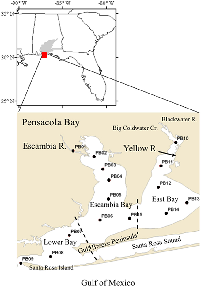
Figure 1. Map of the Pensacola Bay system and sampling sites. Sub-regions of the Bay are delimited by dashed lines between stations PB14 and PB15, which separates East Bay and Escambia Bay, and between PB07 and PB06, which separates Lower Bay and Escambia Bay. The Pensacola Bay watershed is shown in gray in the upper panel.

Watershed Discharges and Concentrations and Loads of Nitrate, Phosphorus, Organic Carbon, and Suspended Solids

Mean daily river discharge rates (Q) for the largest rivers draining to Pensacola Bay were obtained from the U.S. Geological Survey (USGS) for the study period 2003–2012. Discharge data were retrieved for gaging sites on Escambia River (USGS 02376033), Big Coldwater Creek (USGS 02370500), Blackwater River (USGS 02370000) and Yellow River (USGS 02369600; Figure 1). The discharge from the Escambia (mean = 190 m³ s⁻¹) and Yellow rivers (mean = 64 m³ s⁻¹) comprised 91% of the total river discharge (279 m³ s⁻¹) to the bay. The remaining 9% is attributed primarily to the Blackwater River and Big Coldwater Creek, which drain into upper East Bay. Thus, subsequent analyses were restricted to the Escambia and Yellow river data. Because elevated river ${\text{NO}}_3^{-}$ and Chla were observed under low discharge, baseflow conditions (discussed below), we considered whether baseflow loads may be important explanatory variables of estuarine water quality. Daily baseflow discharges (Qb) for Escambia and Yellow rivers were calculated using a hydrograph separation method (Gustard et al., 1992). Briefly, this method consisted of four steps: (1) Divide the daily discharge record into non-overlapping blocks of 5 days and compute the minimum of each block that we call Q₁, Q₂, Q₃,…Q_n. (2) Next we consider the series (Q₁, Q₂, Q₃), (Q₂, Q₃, Q₄),…(Q_i−1, Q_i, Q_i+1). For each series, if 0.9 × center value < outer values, then we save the center value and its date as a point for the baseflow line. This results in a series of values Qb₁, Qb₂, Qb₃, Qb_n with different time periods between them. (3) Linearly interpolate between Qb_i values to estimate daily values of Qb. (4) For the interpolated series, if Qb_i > Q_i then set Qb_i = Q_i.

Observed ${NO}_{\mathit{\text{3}}}^{-}$, total Kjeldahl nitrogen (TKN), total phosphorus (TP), chlorophyll a (Chla_River), total organic carbon (TOC), and total suspended sediment (TSS_River), collected by the Florida Department of Environmental Protection, were obtained from the U.S. water quality portal (https://www.waterqualitydata.us/). Approximately monthly samples were collected at the Escambia River site (21FLBFA_WQX-33020007), which was co-located with the USGS Escambia River discharge gage. Seasonal samples were collected at the Yellow River site (21FLBFA_WQX-33040003), which was co-located with the USGS Yellow River discharge gage.

In order to calculate monthly averages, a rating curve method was applied to observed NO₃⁻, TKN, TP, Chla_River, TOC, and TSS_River observations (Cohn et al., 1989, 1992). The rating curve regression model equation was

$\begin{array}{cc}\begin{array}{l}\ln \left(C\right)={\beta }_0+{\beta }_{1}ln\left(\frac{Q}{Q\prime }\right)+{\beta }_2\left(T-T\prime \right)+{\beta }_3{\left(T-T\prime \right)}^2\\ +{\beta }_4\sin \left(T\right)+\epsilon ,\end{array}& \left(1\right)\end{array}$

where C was a vector of observed constituent concentrations, Q was a vector of daily discharge rates for the dates (T, converted to radians) when C were collected, and Q′ and T′ were centering variables. C and Q were log transformed to obtain normally distributed residuals. β₀, β₁, β₂, β₃, and β₄ were regression coefficients calculated for each regression model and the last term, ϵ, was the error. Using the regression models, daily concentrations for each constituent were calculated for the study period based on the daily observed discharge rates and time. Then, mean monthly and annual discharge and constituent concentrations were calculated from the daily time-series. Finally, monthly and annual constituent loading time-series were calculated as the products of discharges and constituent concentrations.

Derivation of MERIS Chla, CDOM, and TSS

The in situ water quality and optical observations used to develop empirical algorithms for retrieving Chla, CDOM, and TSS from MERIS observations in Pensacola Bay have been described previously (Le et al., 2016; Conmy et al., 2017). Here, a brief summary of the methods is presented for field sampling, laboratory measurements, and validation of satellite observations in comparison to measurements.

Water samples for Chla, CDOM, and TSS analysis (n = 161) were collected from the surface of Pensacola Bay (0.5 m depth) at 15 stations (Figure 1) approximately every 6 weeks from September 2009 to December 2011. Water samples were processed on the day of collection and retained sample filter pads and filtrate were stored at −70°C until analysis. Chla samples were collected on 25 mm GF/F filters (nominal pore size = 0.7 μm), and then, later, extracted from the filter pad with hot methanol and assayed fluorometrically (Welschmeyer, 1994). TSS samples from a measured volume of bay water were collected on pre-weighed, combusted (550°C for 4 h) 47 mm GF/F filters. TSS was measured gravimetrically by drying the sample filter pad (105°C), reweighing, and subtracting the initial filter weight. CDOM in the filtrate obtained from TSS processing was assayed by measuring the specific absorption at 443 nm in a 10-cm quartz cell on a dual-beam scanning spectrophotometer (Shimadzu UV-1700). The absorption spectra from λ = 400–700 nm of dissolved organic matter [ag(λ)] were further measured on the dissolved fraction (Pegau et al., 2003). Absorption spectra from particles [ap(λ)] and non-algal detrital particles [ad(λ)] were quantified on a dual-beam scanning spectrophotometer using the quantitative filter technique (Kiefer and SooHoo, 1982; Kishino et al., 1985). After measuring ap(λ), phytoplankton pigments were extracted from the filter with warm methanol and then the spectra of the filter pad was scanned again to obtain ad(λ). Phytoplankton absorption spectra [aph(λ)] were calculated as the difference between ap(λ) and ad(λ).

Remote sensing reflectance (Rrs) spectral data were measured at each station with a spectroradiometer (HyperSAS, Satlantic Inc., Halifax, Nova Scotia) mounted to the top of the boat, 2 m above the water surface. The HyperSAS collected spectra (1 nm resolution at λ 350–800 nm) of above-water radiance, sky radiance, and downwelling sky irradiance. At each station, An AC-s (Wet-Labs, Philomath, OR) was used to collect vertical water-column profiles of absorption and beam attenuation. Absorption and beam attenuation were measured at 1 nm resolution from 400 to 735 nm. AC-s absorption, attenuation, and calculated scattering spectra were corrected for changes in salinity and temperature, measured with a Seabird CTD (Wet-Labs; Sullivan et al., 2006). AC-s data were averaged from the surface of the water column to the observed Secchi depth and used to correct the R_rs spectra (Gould et al., 1999, 2001).

R_rs bands corresponding with MERIS bands were extracted to calculate empirical algorithms relating observed R_rs to observed Chla (mg m⁻³), CDOM (m⁻¹), and TSS (g m⁻³; Le et al., 2016). Only data collected on cloud-free days and with wind speed < 3 m s⁻¹ were used to develop algorithms. For Chla, the NIR-red band ratio of R_rs(709)/R_rs(665) was selected in order to minimize interference from CDOM and non-algal detritus. For CDOM, the NIR-green band ratio of R_rs(709)/R_rs(510) was used due to uncertainties in the atmospheric correction at blue bands (443 and 490 nm) and interference from phytoplankton absorption in the red bands (665 and 681 nm). For TSS, the band ratio R_rs(709)/R_rs(681) gave the best fit. The equations for the band ratio algorithms were

$\begin{array}{cc}Chla=29.3{\left(\frac{Rrs(709)}{Rrs(665)}\right)}^{4.15},R^2=0.70(n=150)& \left(2\right)\end{array}$

$\begin{array}{cc}CDOM=1.41{\left(\frac{Rrs(709)}{Rrs(510)}\right)}^{0.89},R^2=0.79(n=129)& \left(3\right)\end{array}$

$\begin{array}{cc}TSS=13.9{\left(\frac{Rrs(709)}{Rrs(681)}\right)}^{3.67},R^2=0.71(n=143),& \left(4\right)\end{array}$

where R² were the percentage of variation in the observed data explained by the algorithms and n were the number of samples.

Daily MERIS level-2 data were obtained from NASA (http://oceancolor.gsfc.nasa.gov/) for the study period January 1, 2003 to April, 2012. Downloaded products included MERIS R_rs(λ) in all the spectral bands with 300-m spatial resolution as well as quality control flags for clouds, atmospheric correction warning, and stray light. Pixels along the shoreline with water depths < 2 m were masked to avoid issues with bottom-reflectance. Algorithm Equations (2–4) were then applied to the MERIS R_rs time-series to generate MERIS Chla, CDOM, and TSS time-series. To validate the algorithms, MERIS R_rs(λ) data were extracted for the dates and locations of sampling stations with a time window of ±1 d and calculating a median R_rs(λ) from a 3 × 3 pixel box centered on the sampling location (Le et al., 2013). For subsequent comparisons with river discharge, concentration, and loading time-series, the MERIS Chla, CDOM, and TSS have been averaged to monthly and annual values for the period from January 2003 to December 2011.

Relating River Discharge, Concentrations, and Loads to MERIS Chla, CDOM, and TSS

On a per pixel basis, Pearson correlations among MERIS monthly Chla, CDOM, and TSS time-series and time-series of Q, Qb, river concentrations, and river loads were calculated. We examined correlations with concurrent (0-month), 1-month, and 2-month lagged river time-series. In order to further identify how multivariate combinations of river loads could explain variation in MERIS bio-optical water quality, the MERIS data were averaged over discrete regions, namely Escambia Bay, East Bay, and Lower Bay (Figure 1), and the regional time-series were then regressed against monthly and annual time-series of river loads. We used a partial least squares (PLS) regression model because of the high degree of correlation between independent variables (described below in Results) and because for the annual time-series there were more independent variables (see Equation 5 below) than annual samples (n = 9 years). PLS regression reduces the number of predictor variables by combining the variables into factors similar to principal component analysis. Nine regression models were developed: 3 MERIS water quality variables (i = Chla, CDOM, and TSS) by 3 bay regions (j = Escambia, East, and Lower). The regression equation had the form

$\begin{array}{cc}\begin{array}{l}MERISW{Q}_{ij}~QN{O}_3^{-}+QTKN+QTP+QChl+QTOC\\ +QTSS+QbN{O}_3^{-}+QbTKN+QbTP\\ +QbChl+QbTOC+QbTSS\end{array}& \left(5\right)\end{array}$

where MERIS WQ_ij were the log transformed MERIS water quality time-series per bay region, and variables on the right hand side were the log transformed time-series of river loads (variables beginning with a Q) and baseflow loads (variables beginning with a Qb). For Escambia Bay (j = 1) and Lower Bay (j = 3), the Escambia River loads were used as the independent variables. For East Bay (j = 2), the Yellow River loads were used.

Results

Watershed Discharge, Baseflow, Concentrations, and Loads

Watershed discharge was greatest in the winter and spring in both the Escambia and Yellow rivers (Figure 2). Notable discharge events occurred during April 2005 and December 2009. April 2005 was the wettest month on record at the time for the city of Pensacola, going back to 1880, with 62 cm of rainfall, which resulted in a mean monthly discharge of 768 m³ s⁻¹ for the Escambia River and 283 m³ s⁻¹ for the Yellow River. Escambia River discharge in December 2009 exceeded April 2005 with a monthly average discharge of 883 m³ s⁻¹, while Yellow River discharge was 127 m³ s⁻¹ in December 2009. Overall, for the study period the mean discharges from the Escambia and Yellow rivers were 188 and 68 m³ s⁻¹, respectively. Discharge rates in the two rivers were highly correlated (r = 0.85).

FIGURE 2

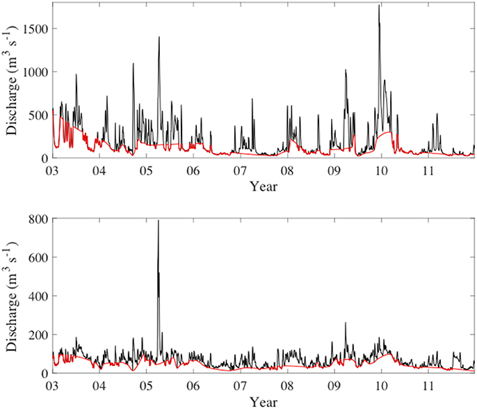
Figure 2. Daily river discharge from the Escambia River (upper) and Yellow River (lower). The red line in both plots shows the calculated baseflow discharge.

Baseflow discharge followed a similar pattern as total discharge with highest baseflow discharge in the winter and spring. For the study period, mean baseflow discharges of the Escambia and Yellow rivers were 109 and 45 m³ s⁻¹, respectively, which represented 75% of the total discharge in the Escambia River and 72% in the Yellow River. During the summer and fall low discharge periods, the baseflow discharge often accounted for all of the observed river discharge (Figure 2). During high discharge periods the baseflow contribution was considerably less. For example, during April 2005 and December 2009, baseflow contributed only 20% and 27%, respectively, of the total discharge from the Escambia River.

Escambia and Yellow river time-series concentrations are shown in Figure 3. On average, concentrations were higher in the Escambia River (Table 1) where mean concentrations for NO₃⁻, TKN, TP, Chla, TOC, and TSS were 15.8 mmol m⁻³, 26.3 mmol m⁻³, 1.17 mmol m⁻³, 1.62 mg m⁻³, 454 mmol m⁻³, and 9.4 g m⁻³, respectively. NO₃⁻ and Chla concentrations in the rivers were negatively correlated with discharge (Table 2). All the other constituent concentrations were positively correlated with discharge. Temporal trends and seasonal patterns were also observed in the data. Significant temporal trends occurred in discharge, NO₃⁻, TP, and TSS (Table 2). Seasonal patterns were observed in Chla and TKN with generally higher values in summer than in winter (Figure 3). These trends formed the basis for our rating curve regression models. All models were statistically significant (p < 0.05) and R² ranged from 0.19 for TSS to 0.76 for ${NO}_{\mathit{\text{3}}}^{-}$.

FIGURE 3

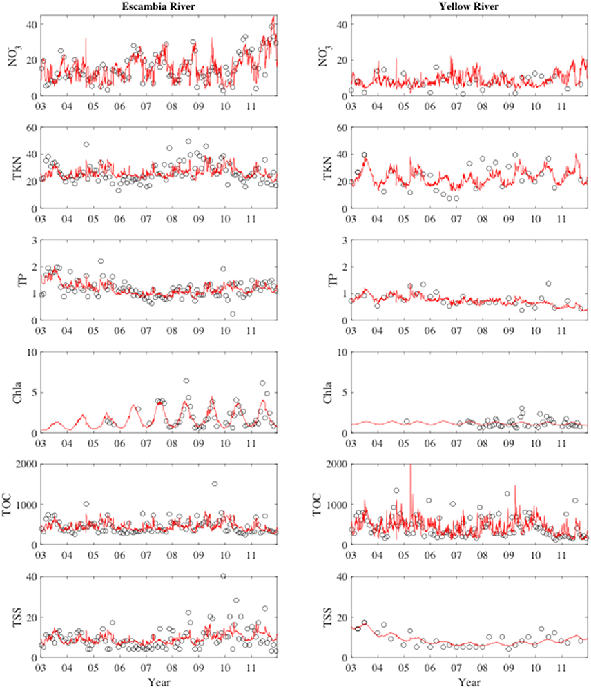
Figure 3. River concentrations during the study period. Left column are the Escambia river time-series and the right column are the Yellow River time-series. Concentration units are mmol m⁻³ for all variables except for Chla (mg m⁻³) and TSS (g m⁻³). The solid red lines in each plot show the rating curve model fits to the observations.

TABLE 1

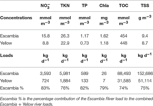
Table 1. Mean river concentrations and loads.

TABLE 2

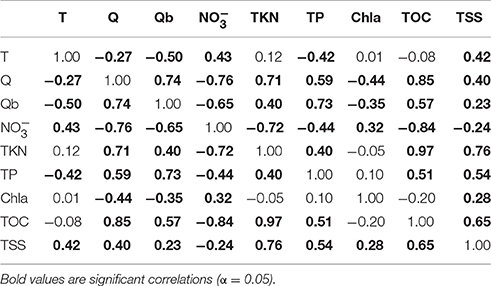
Table 2. Pearson correlation between monthly time (T), river discharge(Q), baseflow discharge (Qb), and concentrations of nitrate (${\text{NO}}_3^{-}$), total Kjeldahl nitrogen (TKN), total phosphorus (TP), chlorophyll a, total organic carbon (TOC), and total suspended sediment (TSS).

River loads to Pensacola Bay were mainly from the Escambia River, which accounted for 74–83% of the total combined constituent loads from Escambia and Yellow rivers (Table 1). Mean Escambia River loads of NO₃⁻, TKN, TP, Chla, TOC, and TSS were 3,593, 5,981, 589, 26, 88,493, and 152,686 kg d⁻¹, respectively. Temporal patterns in river loads generally mimicked the patterns of river discharge (Figure 4).

FIGURE 4

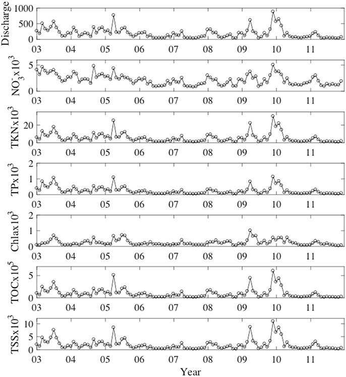
Figure 4. Escambia River monthly mean discharge and loads. River loads of ${\text{NO}}_3^{-}$, TKN, TP, and TOC have units of mmol s⁻¹. Loads of Chla have units of mg s⁻¹ and loads of TSS have units of g s⁻¹.

Pensacola Bay Observed Data and MERIS Algorithms and Time-Series

We briefly summarize the results from Pensacola Bay optical observations and MERIS algorithm development as these results have been presented previously (Le et al., 2016). Rrs was greatest in East Bay and Escambia Bay and smallest in Lower Bay (Figure S1A). For the wavelengths coincident with the MERIS bands used to generate the algorithms in Equations (2–4), spectral absorption was dominated by CDOM at 510 nm, and by a_ph and a_d at 665, 681, and 710 nm (Figures S1B–D).

The band ratio algorithms (Equations 2–4) explained 70%, 79%, and 71% of the variability in Chla, CDOM, and TSS, respectively. Validation results (Figure S2) demonstrate a reasonable accuracy for MERIS derived Chla, CDOM, and TSS where error statistics for Chla were R² = 0.64, MRE = 31.9%, n = 46; for CDOM were R² = 0.80, MRE = 18.5%, n = 53; and for TSS were R² = 0.54, MRE = 42.7%, n = 53. MRE (mean relative error) was calculated by

$\begin{array}{cc}\text{MRE}=\frac{1}{n}{\displaystyle \sum a}bs\left(\frac{MERIS-Observed}{Observed}\right)·100& \left(6\right)\end{array}$

Upon application of these algorithms to the retrieved MERIS reflectance, synoptic monthly time-series of MERIS Chla, CDOM, and TSS were derived. As an example, Figure 5 depicts Chla in the summer and fall during a low discharge year in 2007 and a high discharge year in 2009 (Figure 2). The fall bloom in 2007 had greater Chla than in 2009 despite the lower discharge. This points to other potential mechanisms, besides river forcing, regulating Pensacola Bay Chla such as wind-driven resuspension events (Le et al., 2016).

FIGURE 5

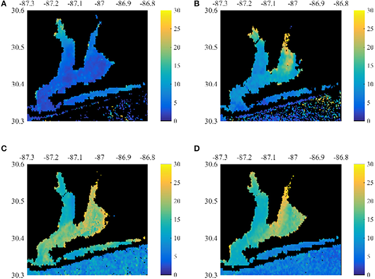
Figure 5. Summer and fall MERIS Chla for the Pensacola Bay system. (A,B) Show the average Chla from August 2007 and August 2009. (C,D) Show the average Chla from October 2007 and November 2009.

After averaging across the bay sub-regions (Figure 1), seasonal patterns in MERIS Chla, CDOM, and TSS were apparent with elevated concentrations in late fall and early winter and lower concentrations in the summer and early fall (Figure 6). MERIS Chla, CDOM, and TSS were highly correlated at monthly (Figure 6) and annual (Figure S3) time scales; monthly Chla and CDOM (r = 0.91); monthly Chla and TSS (r = 0.85), and monthly CDOM and TSS (r = 0.82); annual Chla and CDOM (r = 0.85); annual Chla and TSS (r = 0.79), and annual CDOM and TSS (r = 0.87).

FIGURE 6

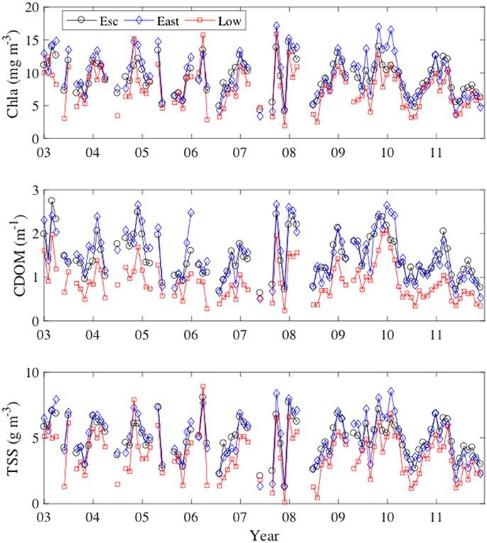
Figure 6. Monthly time-series of MERIS derived Chla, CDOM, and TSS from January 2003 to December 2011.

Relating MERIS Time-Series to River Discharge, Concentration, and Loading Time-Series

Correlation Maps

We examined correlations by pixel between MERIS Chla, CDOM, and TSS time-series and 0-, 1-, and 2-month lagged time-series of Escambia River and Yellow River discharges, concentrations, and loads of NO₃⁻, TKN, TP, Chla, TOC, and TSS. Correlations were similar using either Escambia River or Yellow River data owing to the strong correlation between river discharge for these two rivers (r = 0.85). Thus, as the Escambia River was the largest river input to Pensacola Bay, we present the correlations obtained using the monthly time-series for Escambia River (Figure 4). For correlations with 0-month lagged river forcing, MERIS Chla was most highly correlated with discharge and baseflow discharge (Figure 7). Correlations with river concentrations of NO₃⁻, TP, and TKN were small and correlations with river concentrations of Chla_River were mainly negative. Correlations with river TOC and TSS concentrations (not shown) had similar patterns as for TKN. For 1- and 2-month lagged discharge, baseflow discharge, and river concentrations, MERIS Chla correlations were smaller than for 0-month (not shown).

FIGURE 7

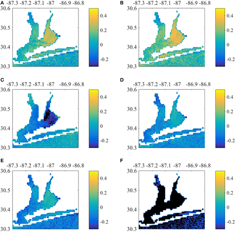
Figure 7. Correlations between monthly Chla time-series (per pixel) with 0-month lagged Escambia River discharge and concentrations. Shown are Chla correlation with (A) discharge, (B) baseflow discharge, and concentrations of (C) river ${\text{NO}}_3^{-}$, (D) river TKN, (E) river TP, and (F) river Chl.

To examine spatial patterns of correlation between MERIS water quality time-series and river loading time-series we focused our analysis on 0-month river loads of NO₃⁻, TP, TOC, and TSS. We included NO₃⁻ and TP as we expected these nutrient loads to be related to bay Chla. We included river TOC as it was expected the load would scale with bay CDOM. Further, TOC and TKN concentrations were highly correlated (r = 0.97). Thus, TOC could act as a surrogate for organic nitrogen. River TSS load was expected to scale with bay TSS.

MERIS Chla had greatest correlation with 0-month lagged NO₃⁻ loads and TOC baseflow loads (Figure 8). East Bay pixels had higher correlation with loading rates than other regions. In contrast, Santa Rosa Sound and the nearshore Gulf of Mexico pixels had higher correlation with 1-month lagged loads (Figure S4). MERIS CDOM also correlated with concurrent NO₃⁻ load and TOC baseflow load (Figure 9). Correlations were apparent throughout Escambia Bay, East Bay, and Lower Bay, although the upper-most reaches of both Escambia and East bays had weak correlation. CDOM correlations with 1-month lagged loads had greater correlation in Santa Rosa Sound and nearshore Gulf of Mexico (Figure S5). MERIS TSS had highest correlation with NO₃⁻ loads, both total and baseflow loads, and with baseflow TOC load (Figure 10). Correlations exhibited similar spatial patterns with highest correlations in East Bay for 0-month loads and in Santa Rosa Sound and nearshore Gulf of Mexico for 1-month loads (Figure S6).

FIGURE 8

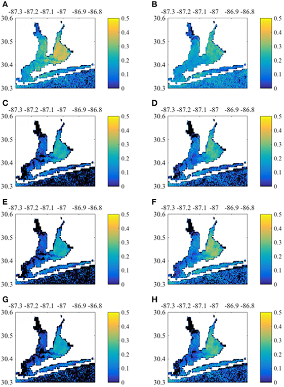
Figure 8. Correlation between monthly Chla time-series per pixel with 0-month lagged Escambia River loads. (A,B) Correlation with ${\text{NO}}_3^{-}$ load and baseflow ${\text{NO}}_3^{-}$ load, respectively. (C,D) Correlation with TP load and baseflow TP load, respectively. (E,F) Correlation with TOC load and baseflow TOC load, respectively. (G,H) Correlation with TSS load and baseflow TSS load, respectively.

FIGURE 9

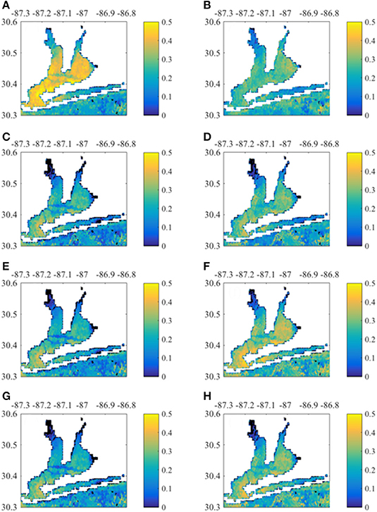
Figure 9. Correlation between monthly CDOM time-series per pixel with 0- month lagged Escambia River loads. (A,B) Correlation with ${\text{NO}}_3^{-}$ load and baseflow ${\text{NO}}_3^{-}$ load, respectively. (C,D) Correlation with TP load and baseflow TP load, respectively. (E,F) Correlation with TOC load and baseflow TOC load, respectively. (G,H) Correlation with TSS load and baseflow TSS load, respectively.

FIGURE 10

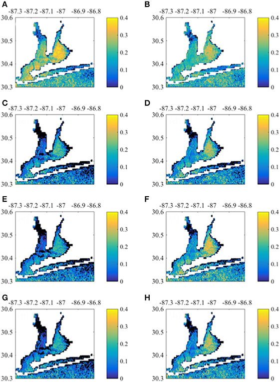
Figure 10. Correlation between monthly TSS time-series by pixel with 0-month lagged Escambia River loads. (A,B) Correlation with ${\text{NO}}_3^{-}$ load and baseflow ${\text{NO}}_3^{-}$ load, respectively. (C,D) Correlation with TP load and baseflow TP load, respectively. (E,F) Correlation with TOC load and baseflow TOC load, respectively. (G,H) Show correlation with TSS load and baseflow TSS load, respectively.

Partial Least Squares Regression Results

At monthly time-scales, the PLS regression models explained 23–59% of the monthly variability in bay water quality (Figure 11). At the annual scale, PLS models explained 20–62% of the variability (Figure 12). By evaluating more parsimonious forms of Equation (5), we determined that that the following reduced equation could represent most of the variability in MERIS Chla, CDOM, and TSS

$\begin{array}{cc}MERISW{Q}_{ij}~QN{O}_3{}^{-}+QTKN+QTSS& \left(7\right)\end{array}$

FIGURE 11

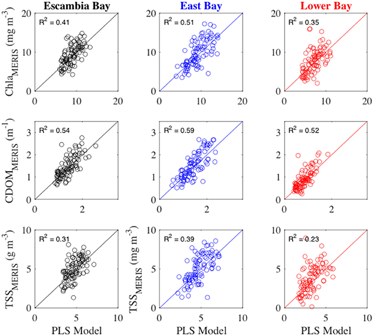
Figure 11. MERIS monthly water quality variables vs. partial least squares regression models (PLS Model). Monthly MERIS water quality time-series for Escambia Bay (left column) and Lower Bay (right column) are compared to the PLS model that was based upon Escambia River monthly loads. Monthly MERIS water quality time-series for East Bay (middle column) are compared to the PLS model that was based upon Yellow River monthly loads. The solid line is the 1:1 line. R² values provide the fraction of variability explained by the PLS models.

FIGURE 12

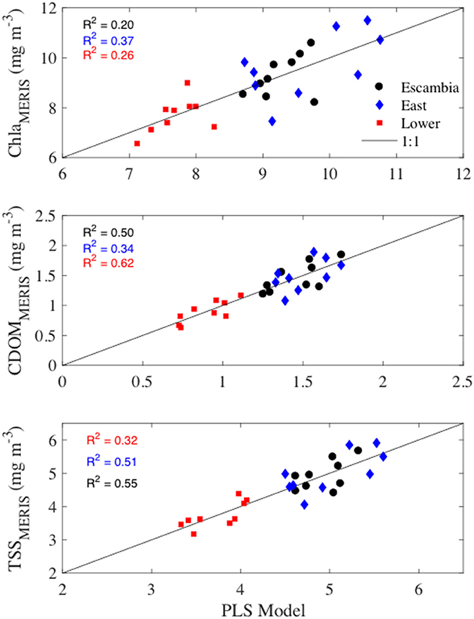
Figure 12. MERIS annual water quality variables vs. partial least squares regression models based upon Escambia River annual loads of ${\text{NO}}_3^{-}$, TKN, and TSS. The solid line is the 1:1 line. R² values provide the fraction of variability explained by the PLS models.

Our justification for this reduced equation was based on several lines of reasoning: (1) the correlation between discharge and baseflow (r = 0.74, Table 2) suggested we could eliminate baseflow loads, (2), the weak correlations of MERIS water quality with either river TP (Figures 8–10) or river Chl (Figure 7F) indicated these loads made an insignificant contribution, and (3) the strong correlation between TKN and TOC (r = 0.97, Table 2) indicated that TKN could be substituted for TOC (discussed further below in Methodological Considerations see Section Methodological Considerations). This reduced form of the model explained 17–56% of the monthly variability in MERIS water quality and 17–62% of the annual variability. Based on Table 3 of PLS component loadings, component 1, which included a linear combination of QTKN and QTSS (equal weights) and ${QNO}_{\mathit{\text{3}}}^{-}$ (lower weight), was the strongest driver of variability in the MERIS Chla, CDOM, and TSS in the three bay regions. Component 2, which had the highest loading from ${QNO}_{\mathit{\text{3}}}^{-}$, also contributed significantly to the total variance explained in East Bay (Table 3), and to a lesser extent in Escambia and East Bay.

TABLE 3

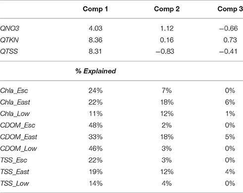
Table 3. Mean PLS loadings for components 1, 2, and 3 of multiple regression model and the percentage of variance explained in the dependent variables.

Discussion

In many estuarine and coastal systems, observational data are insufficient to link estuarine water quality responses to anthropogenic changes in adjacent watersheds. As a supplemental data source, and in some cases the only data source, ocean color satellites are emerging as powerful tools for monitoring and studying estuarine water quality properties that can be measured optically. Previous work has further demonstrated that satellite derived water quality is useful for quantifying the effects of river forcing. Several studies have assessed the responses of satellite-derived estuarine Chla, CDOM, and TSS to variations in river discharge (Acker et al., 2005; Green et al., 2008; Chen et al., 2013; Le et al., 2016) and nutrient loads (Green and Gould, 2008; Chen et al., 2013; Le et al., 2014). To our knowledge, no previous studies have used the satellite data to investigate multivariate relationships between riverine loads of nutrients, organic matter, and sediments and satellite-derived Chla, CDOM, and TSS, nor have previous studies been conducted in small to moderate sized estuaries such as Pensacola Bay (SCOPUS search for keywords: satellite ocean color, estuary, and multivariate water quality on Aug 8, 2017).

MERIS Chla, CDOM, and TSS Relationships to River Forcing

Based on correlation and PLS analyses, the river variables that explained the most variation in MERIS Chla, CDOM, and TSS were Q, Qb, and ${NO}_3^{-}$, TKN, and TSS loads (Figures 7, 8, Table 3). This held true for all regions of the Bay, but in East Bay the influence of ${QNO}_{\mathit{\text{3}}}^{-}$ was greater than in either Escambia or Lower Bay (Table 3). In terms of baseflow river loads, MERIS CDOM and TSS, exhibited correlations with baseflow river loads (Figures 9, 10) but Chla had a muted response to baseflow loads (Figure 8). This latter response is odd given that Chla was modestly correlated to baseflow discharge, especially in East Bay (Figure 7). Overall, though, MERIS Chla, CDOM, and TSS had lower correlations with baseflow loads indicating that the total loads were more important throughout the Pensacola Bay system. We had speculated that baseflow loads may be important because the most elevated river ${NO}_{\mathit{\text{3}}}^{-}$ and Chla concentrations occurred under low discharge, baseflow conditions (Table 2).

Correlations with 1-month lagged loads and baseflow loads of NO₃⁻, TP, TOC, and TSS suggested that East Bay and Santa Rosa Sound had the greatest response to lagged river loads (Figures S4–S6). Highest correlations occurred in nearshore areas around the Gulf Breeze Peninsula and into Santa Rosa Sound. Pixels in the nearshore Gulf of Mexico, outside of Pensacola Bay, also exhibited higher correlations with 1-month lagged watershed loads. The lagoonal region of Santa Rosa Sound and the areas in the nearshore Gulf of Mexico may have longer water residence times than other regions of Pensacola Bay owing to the lack of direct river discharges. The nearshore Gulf region may be responding to outflows from Pensacola Bay or to larger regional scale (northern Gulf watersheds) loading to the coastal zone.

PLS regression models based on ${QNO}_{\mathit{\text{3}}}^{-}$, QTKN, and QTSS were relatively good predictors of MERIS Chla, CDOM, and TSS in the three bay regions at both monthly (Figure 11) and annual (Figure 12) time scales. For Pensacola Bay, these empirical models provide a means to evaluate how changes in nitrogen and suspended loads may impact Chla, CDOM, and TSS. Such an analysis is beyond the scope of the present study, but may be of interest for managers who need to determine loading reductions required to achieve water quality targets in the bay. Furthermore, the covariations exhibited among MERIS Chla, CDOM, and TSS in the three bay regions (Figure 6) indicate that load reductions aimed at reducing Chla, CDOM, and TSS are likely to be effective across the entire Bay.

There are few previous studies relating river forcing to field-based observations of water quality in Pensacola Bay. One study found a similar pattern of increased Chla in the bay as a result of increased river discharge (Murrell et al., 2007). Studies of nutrient limitation have resulted in mixed results. In one study, phosphorus limitation of primary production was observed based on nutrient and phosphorus addition experiments at two sites, one in an oligohaline and one in a mesohaline region of the bay (Murrell et al., 2002). In another study, nitrogen limitation of primary production was reported from one polyhaline site in Santa Rosa Sound (Juhl and Murrell, 2008). In the present study, river nitrogen (${NO}_{\mathit{\text{3}}}^{-}$ and TKN) loads explained most of the variability in MERIS Chla as well as in CDOM and TSS, and, thus, supported nitrogen as being more important as a limiting nutrient. Neither river concentrations nor loads of TP were significantly correlated with Chla (Figures 7D, 8D).

In the present study we did not examine the effects of wind on water quality patterns. However, previously wind speed was observed to be significantly correlated (positive) to the MERIS water quality variables in Escambia Bay and East Bay, but not in lower Bay, but correlations were weak (r < 0.29) at a monthly scale (Le et al., 2016). Thus, the percentage of variation explained by the PLS regressions for Escambia and East bays could be improved by including wind as an independent variable for these regions of the bay.

Methodological Considerations

There are several potential errors in our analysis. First of these was the accuracy of the MERIS satellite-derived Chla, CDOM, and TSS. While the algorithms used here appeared to be robust (Section Pensacola Bay Observed Data and MERIS Algorithms and Time-Series), the mean relative errors between field observations and satellite-derived values were 18.5% for CDOM, 31.9% for Chla, and 42.7% for TSS. In coastal waters, further work is required to improve the algorithms that equate remote sensing reflectance and other optical properties to water quality variables.

A second source of potential error was from the strong correlations between river discharges and concentrations (Table 2). For example, TKN and TOC were highly correlated (r = 0.97). These correlations dictated our use of PLS regression when relating monthly and annual river time-series to MERIS water quality. Though PLS is an alternative to typical least squares regression when independent variables are highly correlated, the interpretation of the PLS results is not straightforward. For example, due to the correlation between TKN and TOC we could have used TOC loads in Equation (7) instead of TKN loads with little change in the percent variance explained in the dependent water quality variables. Further, there was a high degree of covariation between monthly time-series of MERIS Chla, CDOM, and TSS as observed in Figure 6, which limits our ability to tease apart the factors controlling these variables. For example, high CDOM or TSS may limit light availability for phytoplankton photosynthesis and in turn limit Chla concentration, yet at the same time Chla, CDOM and TSS were all correlated with nitrogen loading, thus light limitation did not appear to have a significant impact on Chla in surface waters in comparison to the effect of nitrogen loads.

A third issue was the choice of averaging the river and satellite data to a monthly time scale. We chose this averaging period for the practical reason that there may be large gaps in the satellite record at the daily time step due to cloud cover and/or other quality control issues. Also, the river concentration data were collected at monthly to seasonal scales. Averaging at the monthly scale, however, may obscure estuarine patterns related to episodic events such as a tropical storms (Hagy et al., 2006) or peak river discharges (Murrell et al., 2007) that can rapidly flush Pensacola Bay. In future studies, the issue of obtaining greater temporal sampling from satellite may be overcome by including data from other ocean color satellites such as MODIS. A challenge to blending these products is the development of algorithms for each satellite. Including MODIS data in our analysis of Pensacola Bay may not have worked since the spatial resolution and wavelengths of reflectance captured by MODIS are different than MERIS. The greater spatial resolution of MERIS (300 m vs. 1 km for MODIS) and the unique spectral band at 709 nm was the reason that MERIS was applied to Pensacola Bay (Le et al., 2016).

Conclusions and Future Directions

In this study, we demonstrated the utility of long-term and spatially synoptic satellite data for examining the effects of river forcing on estuarine water quality. This is the first study to apply a multi-variate approach to examine this problem and first to do so with MERIS in small to moderate size estuary, Pensacola Bay. The approach to retrieve water quality from MERIS and to analyze the factors driving water quality variability are readily portable to other similar sized estuaries globally. Our primary conclusion was that MERIS Chla, CDOM, and TSS dynamics observed in Pensacola Bay were significantly related to riverine nitrogen loads. However, the analyses also indicated that some of the sub-regions of the bay had different responses to the magnitude and timing of river loads. Overall, the MERIS data provided unprecedented spatial and temporal coverage beyond that of past boat-based efforts in Pensacola Bay and revealed previously unobserved spatial and temporal patterns of responses to river forcing.

A similar approach to the one used in this study could also be applied to water column light absorption and attenuation, which are related measures of water clarity. Improving water clarity is a common water quality goal in Florida estuaries for both ecological and economic reasons. Water clarity is a key ecological attribute in Pensacola Bay that controls primary production (Murrell et al., 2009) and likely the spatial distribution of seagrass habitats in the bay. The MERIS-derived water quality variables used in this study could be applied to better understand controls on water clarity. Chla and TSS scale to the inherent optical properties a_ph and a_d, respectively, in Pensacola Bay (Conmy et al., 2017), and, thus, as CDOM (a_g) is already measured in units of absorption (m⁻¹), it is possible to construct a total absorption (a_t) budget by summing a_ph (obtained by converting from Chla), a_d (obtained by converting from TSS), and a_g. Also, as a_t is linearly related to light attenuation (m⁻¹, Conmy et al., 2017), it will be possible in future work to extrapolate the MERIS derived Chla, CDOM, and TSS to water clarity targets such as percent of surface solar radiation required to support seagrass habitats.

Author Contributions

JL conceived the study, performed data analyses, and wrote the manuscript. CL developed the satellite algorithms, generated the satellite time-series data, and provided comments and edits to manuscript drafts.

Funding

Funding for this work was provided by NASA Applied Science Grant number NNH10AN14I and the U.S. EPA Safe and Sustainable Water Resources Research Program.

Conflict of Interest Statement

The authors declare that the research was conducted in the absence of any commercial or financial relationships that could be construed as a potential conflict of interest.

Acknowledgments

The authors acknowledge J. Aukamp, D. Beddick, R. Conmy, A. Duffy, G. Craven, B. Jarvis, B. Schaeffer, and D. Yates for their contributions to the collection, analysis, and management of the Pensacola Bay optical data. The authors thank the three reviewers and the editor for constructive comments that improved this manuscript.

Supplementary Material

The Supplementary Material for this article can be found online at: https://www.frontiersin.org/article/10.3389/fmars.2017.00274/full#supplementary-material

References

Acker, J. G., Harding, L. W., Leptoukh, G., Zhu, T., and Shen, S. (2005). Remotely-sensed chl α at the Chesapeake Bay mouth is correlated with annual freshwater flow to Chesapeake Bay. Geophys. Res. Lett. 32:L05601. doi: 10.1029/2004GL021852

CrossRef Full Text | Google Scholar

Borkman, D. G., and Smayda, T. J. (1998). Long-term trends in water clarity revealed by Secchi-disk measurements in lower Narragansett Bay. ICES J. Mar. Sci. 55, 668–679. doi: 10.1006/jmsc.1998.0380

CrossRef Full Text | Google Scholar

Boynton, W., Kemp, W., and Keefe, C. (1982). “A comparative analysis of nutrients and other factors influencing estuarine phytoplankton production,” in Estuarine Comparisons, ed V. S. Kennedy (New York, NY: Academic Press), 69–90.

Google Scholar

Bricker, S. B., Clement, C. G., Pirhalla, D. E., Orlando, S. P., and Farrow, D. R. (1999). National estuarine Eutrophication Assessment: Effects of Nutrient Enrichment in the Nation's Estuaries. US National Oceanographic and Atmospheric Administration, National Ocean Service, Special Projects Office and the National Center for Coastal Ocean Science.

Caffrey, J. M., and Murrell, M. C. (2016). “A Historical Perspective on Eutrophication in the Pensacola Bay Estuary, FL, USA,” in Aquatic Microbial Ecology and Biogeochemistry: A Dual Perspective, eds P. Glibert and T. Kana (Cham: Springer), 199–213.

Google Scholar

Chen, C., Jiang, H., and Zhang, Y. (2013). Anthropogenic impact on spring bloom dynamics in the Yangtze River Estuary based on SeaWiFS Mission (1998–2010) and MODIS (2003–2010) observations. Int. J. Remote Sens. 34, 5296–5316. doi: 10.1080/01431161.2013.786851

CrossRef Full Text | Google Scholar

Cohn, T. A., Caulder, D. L., Gilroy, E. J., Zynjuk, L. D., and Summers, R. M. (1992). The validity of a simple statistical model for estimating fluvial constituent loads: an empirical study involving nutrient loads entering Chesapeake Bay. Water Resour. Res. 28, 2353–2363. doi: 10.1029/92WR01008

CrossRef Full Text | Google Scholar

Cohn, T. A., Delong, L. L., Gilroy, E. J., Hirsch, R. M., and Wells, D. K. (1989). Estimating constituent loads. Water Resour. Res. 25, 937–942. doi: 10.1029/WR025i005p00937

CrossRef Full Text

Conmy, R. N., Schaeffer, B. A., Schubauer-Berigan, J., Aukamp, J., Duffy, A., Lehrter, J. C., et al. (2017). Characterizing light attenuation within Northwest Florida Estuaries: implications for RESTORE Act water quality monitoring. Mar. Pollut. Bull. 114, 995–1006. doi: 10.1016/j.marpolbul.2016.11.030

PubMed Abstract | CrossRef Full Text | Google Scholar

Gould, R., Arnone, R., and Sydor, M. (2001). Absorption, scattering, and, remote-sensing reflectance relationships in coastal waters: testing a new inversion algorith. J. Coast. Res. 328–341.

Google Scholar

Gould, R. W., Arnone, R. A., and Martinolich, P. M. (1999). Spectral dependence of the scattering coefficient in case 1 and case 2 waters. Appl. Opt. 38, 2377–2383. doi: 10.1364/AO.38.002377

PubMed Abstract | CrossRef Full Text | Google Scholar

Green, R. E., and Gould, R. W. (2008). A predictive model for satellite-derived phytoplankton absorption over the Louisiana shelf hypoxic zone: effects of nutrients and physical forcing. J. Geophys. Res. 113:C06005. doi: 10.1029/2007JC004594

CrossRef Full Text | Google Scholar

Green, R. E., Gould, R. W., and Ko, D. S. (2008). Statistical models for sediment/detritus and dissolved absorption coefficients in coastal waters of the northern Gulf of Mexico. Cont. Shelf Res. 28, 1273–1285. doi: 10.1016/j.csr.2008.02.019

CrossRef Full Text | Google Scholar

Gustard, A., Bullock, A., and Dixon, J. (1992). Low Flow Estimation in the United Kingdom. Institute of Hydrology.

Hagy, J. D., Lehrter, J. C., and Murrell, M. C. (2006). Effects of hurricane Ivan on water quality in Pensacola Bay, Florida. Estuaries and Coasts 29, 919–925.

Google Scholar

Hagy, J. D., and Murrell, M. C. (2007). Susceptibility of a northern Gulf of Mexico estuary to hypoxia: an analysis using box models. Estuar. Coast. Shelf Sci. 74, 239–253. doi: 10.1016/j.ecss.2007.04.013

CrossRef Full Text | Google Scholar

Handley, L., Altsman, D., and DeMay, R. (2007). “Seagrass Status and Trends in the Northern Gulf of Mexico: 1940-2002.” US Geological Survey.

Harding, L. Jr., Gallegos, C., Perry, E., Miller, W., Adolf, J., Mallonee, M., et al. (2016). Long-term trends of nutrients and phytoplankton in Chesapeake Bay. Estuar. Coasts 39, 664–681. doi: 10.1007/s12237-015-0023-7

CrossRef Full Text | Google Scholar

Juhl, A. R., and Murrell, M. C. (2008). Nutrient limitation of phytoplankton growth and physiology in a subtropical estuary (Pensacola Bay, Florida). Bull. Mar. Sci. 82, 59–82.

Google Scholar

Kiefer, D. A., and SooHoo, J. B. (1982). Spectral absorption by marine particles of coastal waters of Baja California. Limnol. Oceanogr. 27, 492–499. doi: 10.4319/lo.1982.27.3.0492

CrossRef Full Text | Google Scholar

Kishino, M., Takahashi, M., Okami, N., and Ichimura, S. (1985). Estimation of the spectral absorption coefficients of phytoplankton in the sea. Bull. Mar. Sci. 37, 634–642.

Google Scholar

Le, C., Hu, C., English, D., Cannizzaro, J., Chen, Z., Feng, L., et al. (2013). Towards a long-term chlorophyll-a data record in a turbid estuary using MODIS observations. Prog. Oceanogr. 109, 90–103. doi: 10.1016/j.pocean.2012.10.002

CrossRef Full Text | Google Scholar

Le, C., Lehrter, J. C., Hu, C., Murrell, M. C., and Qi, L. (2014). Spatiotemporal chlorophyll-a dynamics on the Louisiana continental shelf derived from a dual satellite imagery algorithm. J. Geophys. Res. 119, 7449–7462. doi: 10.1002/2014JC010084

CrossRef Full Text | Google Scholar

Le, C., Lehrter, J. C., Hu, C., Schaeffer, B., MacIntyre, H., Hagy, J. D., et al. (2015). Relation between inherent optical properties and land use and land cover across Gulf Coast estuaries. Limnol. Oceanogr. 60, 920–933. doi: 10.1002/lno.10065

CrossRef Full Text | Google Scholar

Le, C., Lehrter, J. C., Schaeffer, B. A., Hu, C., Murrell, M. C., Hagy, J. D., et al. (2016). Bio-optical water quality dynamics observed from MERIS in Pensacola Bay, Florida. Estuar. Coast. Shelf Sci. 173, 26–38. doi: 10.1016/j.ecss.2016.02.003

CrossRef Full Text | Google Scholar

Lehrter, J. C. (2008). Regulation of eutrophication susceptibility in oligohaline regions of a northern Gulf of Mexico estuary, Mobile Bay, Alabama. Mar. Pollut. Bull. 56, 1446–1460. doi: 10.1016/j.marpolbul.2008.04.047

PubMed Abstract | CrossRef Full Text | Google Scholar

Monbet, Y. (1992). Control of phytoplankton biomass in estuaries: a comparative analysis of microtidal and macrotidal estuaries. Estuar. Coasts 15, 563–571. doi: 10.2307/1352398

CrossRef Full Text | Google Scholar

Murrell, M. C., Campbell, J. G., Hagy, J. D., and Caffrey, J. M. (2009). Effects of irradiance on benthic and water column processes in a Gulf of Mexico estuary: Pensacola Bay, Florida, USA. Estuar. Coast. Shelf Sci. 81, 501–512. doi: 10.1016/j.ecss.2008.12.002

CrossRef Full Text | Google Scholar

Murrell, M. C., Hagy, J. D., Lores, E. M., and Greene, R. M. (2007). Phytoplankton production and nutrient distributions in a subtropical estuary: importance of freshwater flow. Estuar. Coasts 30, 390–402. doi: 10.1007/BF02819386

CrossRef Full Text | Google Scholar

Murrell, M. C., Stanley, R. S., Lores, E. M., DiDonato, G. T., Smith, L. M., and Flemer, D. A. (2002). Evidence that phosphorus limits phytoplankton growth in a Gulf of Mexico estuary: Pensacola Bay, Florida, USA. Bull. Mar. Sci. 70, 155–167.

Google Scholar

Pegau, S., Zaneveld, J. R. V., Mitchell, B. G., Mueller, J. L., Kahru, M., Wieland, J., et al. (2003). Ocean Optics Protocols for Satellite Ocean Color Sensor Validation, revision 4, Volume IV: INHERENT Optical Properties: Instruments, Characterizations, Field Measurements and Data Analysis Protocols. NASA Tech. Memo 211621.

Sullivan, J. M., Twardowski, M. S., Zaneveld, J. R. V., Moore, C. M., Barnard, A. H., Donaghay, P. L., et al. (2006). Hyperspectral temperature and salt dependencies of absorption by water and heavy water in the 400-750 nm spectral range. Appl. Opt. 45, 5294–5309. doi: 10.1364/AO.45.005294

PubMed Abstract | CrossRef Full Text | Google Scholar

Welschmeyer, N. A. (1994). Fluorometric analysis of chlorophyll a in the presence of chlorophyll b and pheopigments. Limnol. Oceanogr. 39, 1985–1992. doi: 10.4319/lo.1994.39.8.1985

CrossRef Full Text | Google Scholar

Yarbro, L. A., and Carlson, P. (2013). “Seagrass integrated mapping and monitoring program,” in Mapping and Monitoring Report No. 1. Florida. (Fish and Wildlife Research Institute).

Google Scholar