Explanatory Power of Human and Environmental Pressures on the Fish Community of the Grand Bank before and after the Biomass Collapse

Introduction

Marine fisheries collapses worldwide have important socio-economic and ecological consequences, highlighting the need for ecosystem based fisheries management (EBFM; e.g., Misund and Skjoldal, 2005; DFO, 2007). EBFM supplements conventional single species approaches by explicitly considering interactions among species (target and non-target) in the context of changing human activities and environmental conditions. Implementation of EBFM requires information about the whole ecosystem, which can be provided in part by data-based indicators, i.e., measured or derived proxies of biological status and ecological pressures (Larkin, 1996; Jennings, 2005). Biological indicators include measures of the fish community structure (e.g., biomass, mean length, and trophic level of the community). Both fishing and the environment are external pressures on the fish community, and can be quantified by a range of indicators (e.g., Link et al., 2010b; Shannon et al., 2010). Fishing indicators can refer to metrics of landings (e.g., total or species aggregates), effort (e.g., hours fished), and fishing mortality (e.g., landings/community biomass), while environmental indicators can include large-scale metrics of atmospheric forcing, such as the North Atlantic Oscillation (NAO), and region-specific features such as annual mean temperature and salinity. Managers can regulate (at least partially) fishing pressures, but not environmental pressures (on relevant timescales; Elliott, 2011), and yet their decisions must account for future changes in the environment. It is generally accepted that a suite of indicators from several categories (e.g., biological, fishing, and environmental) is required for successful EBFM (e.g., Jennings, 2005; Link et al., 2010b). Considerable effort has focussed on determining which of the hundreds of proposed biological indicators are the most informative (Rice, 2003; Jennings, 2005; Rice and Rochet, 2005; Shin et al., 2010), but there remains a pressing need to determine which sets of pressures are best predictors of change (e.g., Ojaveer and Eero, 2011; Large et al., 2015).

Improving scientific understanding of multivariate pressure-response relationships can contribute to implementation of EBFM. Identifying which pressures are most directly related to changes in the fish community can help focus investigations of thresholds, guide modeling, plan management scenarios, and direct monitoring efforts. Determining which pressures are the most informative is challenging because of the range ways to quantify them, and because the mechanistic relationships are currently not well-defined. For example, there has been fierce debate about whether fishing or poor environmental conditions caused the infamous collapse of cod and other species on the Grand Banks in the 1990s (e.g., Myers et al., 1996; Bundy, 2001; Halliday and Pinhorn, 2009). Furthermore, changes in pressures can have both immediate and delayed effects on fish communities (e.g., Greenstreet et al., 2011; Gröger and Fogarty, 2011; Dempsey et al., 2017), adding an additional layer of complexity to the analysis of pressures and biological responses. For example, immediate effects of fishing include the removal of biomass, while delayed effects include changes in the size structure of the community (Daan et al., 2005; Devine et al., 2007). While previous studies have acknowledged delays (e.g., Chen and Ware, 1999; Large et al., 2015), more investigation into appropriate types and lengths of delays is warranted (Large et al., 2015).

Our objective here was to identify sets of pressures most directly related to three decades of changes in the structure of the fish community of the Grand Bank, Northwest Atlantic (Figure 1). This will add to the current understanding of this ecosystem, while demonstrating a method that could be useful to scientists and managers for other areas. This region provides a valuable case study because it experienced complex ecological changes resulting in two distinct periods, which are spanned by our suite of indicators (Dempsey et al., 2017). We identify pressure indicators from within this suite that can best predict fish community state over the full time series as well as for the two periods, and use our analysis to examine the past and present dynamics of this ecosystem. We also investigate models with different delay lengths (0–5 years) and types (moving average and lags) to determine which delays have the best explanatory power.

FIGURE 1

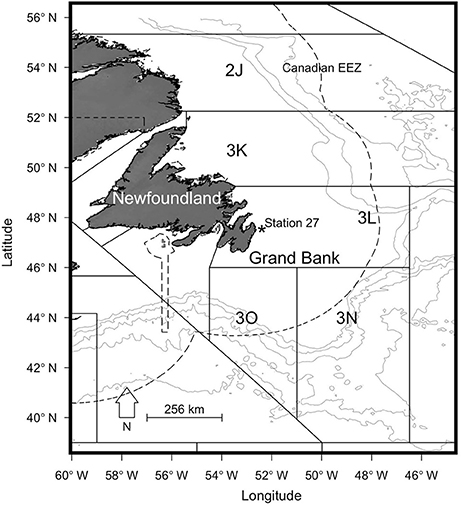
Figure 1. Map of the study area, showing the Grand Bank (NAFO division 3LNO), Station 27, and the Canadian exclusive economic zone (dashed lines).

Methods

Study Area

Here we provide historical context for our study area to highlight some of the ecological changes that have occurred in the region over our period of interest. The Grand Bank, within the Northwest Atlantic Fisheries Organization (NAFO) statistical division 3LNO, and the adjacent southern Labrador and northeast Newfoundland shelf (NAFO Division 2J3K) are recognized as major subunits within the Newfoundland-Labrador shelf in the Northwest Atlantic (Figure 1; NAFO, 2014). The shelf is partly within the Canadian exclusive economic zone (EEZ) established in 1977, but extends into international waters (Figure 1).

For centuries, this region was one of the most productive fishing grounds in the world, with global fisheries for many species including Atlantic cod, flounder, and capelin (Rose, 2007). Fisheries management in the region is the responsibility of Fisheries and Oceans Canada (DFO) within the EEZ, and NAFO in international waters. Throughout the 1980s the primary management strategy for both DFO and NAFO was to set independent quotas for each fish stock; however, these measures were largely ineffective because the limits were ignored by some vessels, and there was error in calculating sustainable exploitation rates (e.g., Rose, 2007). In the 1990s prolonged heavy fishing pressure combined with an environmental regime shift precipitated complex ecological changes, characterized by a collapse of fish biomass. This is commonly referred to as “the collapse of the cod” even though many other species were also impacted (e.g., Atkinson, 1994; NAFO, 2010b). In response to the low biomass of many stocks, groundfish moratoria were enforced for 2J3KL in 1994 and the southern Grand Bank in 1994. Harvesters adapted by targeting different species (e.g., shrimp and crab), retiring from fishing, or leaving the province to find other employment (e.g., Hamilton and Butler, 2001). Over 20 years after imposition of these moratoria, many remain in place (see Annex I.A in NAFO, 2017). The total fish biomass has recovered slowly, although different species are recovering at different rates such that the structure of the ecosystem has shifted from piscivore dominated to include more species at lower trophic levels (Figure 2; Pedersen et al., 2017).

FIGURE 2

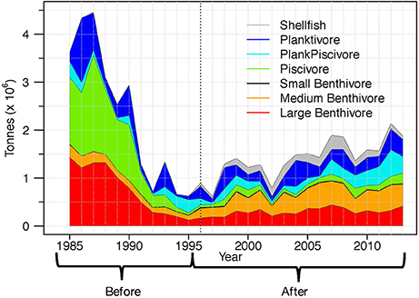
Figure 2. Fish functional group biomass in NAFO division 3LNO, illustrating the collapse of total biomass and changing structure of the community. All functional groups except shellfish are included as response variables. The Before period is from 1985 to 1995, the After period is from 1996 to 2013, and the Full period includes 1985–2013 (Before + After).

Both DFO and NAFO are working toward ecosystem approaches to management (Oceans Act, 1996; DFO, 2009; NAFO, 2010a,b). Current management strategies include the At-Sea Observer Program (DFO, 2014), National Vessel Monitoring System (DFO, 2016), restrictions on total allowable catches (e.g., for redfish and yellowtail flounder; NAFO, 2017), gear restrictions, and restricted entry programs.

Indicators

The indicator time series used here were synthesized and presented in Dempsey et al. (2017). Fish community indicators are annual values for 1985–2013, and pressures used to predict them additionally extend to 1980–1984 for use with our time delay analysis. Below we present a general overview of these indicators to facilitate the reader's appreciation of our current multivariate analysis, and refer interested readers to Dempsey et al. (2017) for more details on indicator trends and data sources.

Indicators of Fish Community Status

The structure of the fish community was represented by the mean annual biomass indices of six fish functional feeding groups (aggregated species), which have been analyzed by Dempsey et al. (2017) and others (e.g., NAFO, 2010b, 2014; Table 1). Such functional groups are meaningful units to fisheries scientists and managers (NAFO, 2014), are compatible with modern ecosystem models (e.g., Link et al., 2010a; Heymans et al., 2016), and benefit the present analysis by reducing the number of response variables when compared to the use of individual species (Fogarty, 2014). The annual biomass index of each functional group was calculated from DFO spring scientific bottom trawl surveys for NAFO area 3LNO by summing the average catch per tow of the species included in the group. In 1996, the survey gear changed from a commercial Engels to a finer-meshed Campelen trawl, such that the biomass indices cannot be directly compared before and after the gear change due to differing capture efficiencies (McCallum and Walsh, 1997; Belgrano and Fowler, 2011). Scaling factors have been developed to coarsely compare the Engels and Campelen biomasses for most species; however, it was not possible to scale the biomasses of invertebrate species (i.e., shellfish) because they were not sampled consistently by the Engels trawl (Koen-Alonso, unpublished data).

TABLE 1

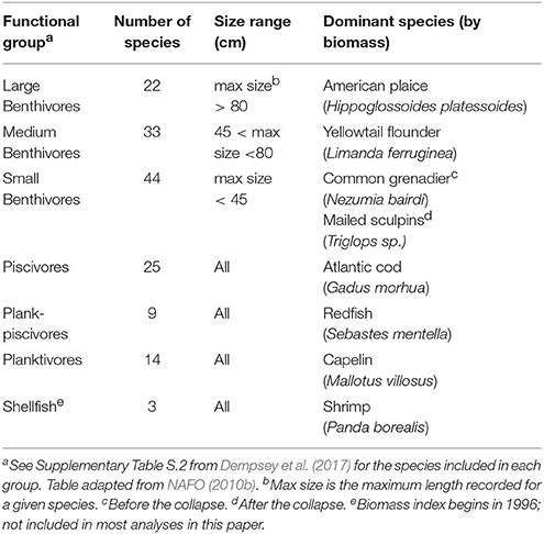
Table 1. Functional groups used to represent the fish community structure of the Grand Bank, Newfoundland.

The mid-1990s also correspond to the minimum total fish biomass in the region, marking the end of the rapid collapse of biomass and the beginning of the recovery. These have been characterized as two ecologically different periods (e.g., Buren et al., 2014; Dempsey et al., 2017). Here we analyzed three time periods: the Full period (1985–2013; using the scaled Engels data) as well as Before (1985–1995) and After (1996–2013) the collapse. “Before” and “After” also correspond to the survey gear change to eliminate the reliance on the coarse scaling factors. Note that because there is no appropriate biomass index for shellfish prior to 1996 (NAFO, 2010b), this functional group had to be excluded from the Full and Before analyses. We do not expect this exclusion to affect results because even though the build-up of shrimp (the major species by biomass in this group) is believed to have started in the mid 1980s, it only peaked on the Grand Bank in the 2000s (Lilly et al., 2000; NAFO, 2014). As discussed later, some After analyses were completed with and without the shellfish index to determine the effect of including this functional group.

Indicators of Fishing and Environmental Pressures

The nine pressure indicators chosen as predictors for this analysis were based on the results of Dempsey et al. (2017; Figure 3). Note that we do not distinguish “pressures” from “drivers,” as some authors do (e.g., in the DPSIR framework, see Gari et al., 2015 and references therein), because they both ultimately influence the fish community and as such it would be a matter of semantics for this analysis.

FIGURE 3

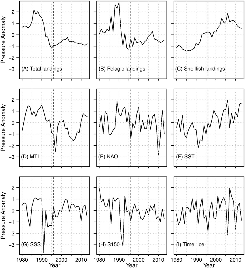
Figure 3. Pressure indicators used as predictors in this analysis. Fishing indicators: (A–D); Environmental indicators: (E–I). The thick dashed line indicates the beginning of the After period.

Four fishing indicators were included (Figure 3): total, pelagic, and shellfish landings, as well as the marine trophic index (MTI; denoted “MTI_Land” in Dempsey et al., 2017). Total landings are the sum of groundfish, pelagic, shellfish, and “other” species landings, and provide a metric of fishing pressure on the entire community. Pelagic landings are dominated by capelin, which is a key forage species in the system, and shellfish landings are dominated by shrimp and queen crab (also known as snow crab). MTI is the mean trophic level of the landings weighted by the biomass of species landed, including only species with trophic level ≥ 3.25 (e.g., Atlantic cod, haddock). MTI reflects evolving fishing practices as fishers target different species to adapt to changes in fishing technologies, the ecosystem, and end markets (Caddy and Garibaldi, 2000).

In general, the fishing indicators were highly correlated Before the collapse and for the Full period (Pearson correlation coefficient > 0.60, not shown), but not After the collapse (not shown). Total and pelagic landings both increased in the early 1980s, and then decreased from the late 1980s until the mid-1990s, and to this day remain lower than in the late 1970s and 1980s. MTI also decreased throughout the Before period, but has no trend in the After. Shellfish landings increased over the Full period due to the proliferation of shrimp and crab stocks in the 1980s and a shift in target species after the groundfish moratoria (Schrank, 2005; Dempsey et al., 2017), but have been declining since the mid-2000s (Figure 3; Department of Fisheries Aquaculture, 2014; Dempsey et al., 2017).

Five environmental indicators were included as predictors (Figure 3): the North Atlantic Oscillation (NAO), sea surface salinity (SSS), salinity at 150 m (S150), sea surface temperature (SST), and the timing of the sea ice melt (Time_Ice). The NAO represents basin scale atmospheric circulation patterns that influence winds, salinity, temperature, and sea ice (Hurrell, 1995; Petrie, 2007). The remaining indicators characterize physical environmental factors local to the Grand Bank, which are thought to have played a critical role in the collapse of fish biomass in the 1990s (e.g., Halliday and Pinhorn, 2009). Time_Ice was included as a proxy of the timing of the spring phytoplankton bloom (Wu et al., 2007) because there are no other suitable measures of phytoplankton biomass or productivity over the required historical time frame.

In general, the environmental pressures were not highly correlated with each other or the fishing pressures for any period (not shown). SST was the only environmental pressure with clear trends: it decreased until 1991, and has generally increased since. The remaining indicators were characterized by inter-annual variability. Notably, the NAO was well above its average in the early 1990s, leading to cooler and fresher water at this time, which has been characterized as a regime shift (Buren et al., 2014). The salinity indicators had higher variability Before the collapse, with extreme minimum values in the mid-1990s. In contrast, Time_Ice had higher variability After the collapse (Figure 3).

Method of Data Analysis

Redundancy Analysis

Redundancy analysis (RDA) was used to assess how well different sets of the pressures described above simultaneously modeled the biomasses of all six functional groups over a period of n years. RDA is a multivariate extension of linear regression that uses p predictors in matrix X_{[n x p]} to model r responses in matrix Y_{[n x r]}. The explanatory power is characterized using goodness of fit metrics related to variances in the responses, the model, and/or the residuals. Commonly used metrics are the coefficient of determination (R²) and the adjusted-R². The R² measures the fraction of the total variance in the response(s) that is explained by the variance in predictor matrix X. The adjusted-R² is a modification to R², which enables comparison among models using different numbers of predictors (see below; Legendre and Legendre, 2012).

The first step in RDA is a multiple linear regression of each response variable (r multiple regressions), which are typically done simultaneously for computational efficiency. The modeled values are stored in the matrix Ŷ_{[n x r]}, while matrix $\widehat{\beta }$_{[p x r]} holds the coefficients for linear combinations of the columns of X, and result in the smallest sum of squares of the residuals for each response:

$\begin{array}{ll}\widehat{\text{Y}}=\text{X}\widehat{\beta }=\text{X}{\left({\text{X}}^{\text{T}}\text{X}\right)}^{-1}{\text{X}}^{\text{T}}\text{Y}& (1)\end{array}$

where the superscript symbols “T” and “−1” respectively denote the matrix transpose and inverse. It is assumed that the columns of X are linearly related to the columns of Y, and so appropriate transformations must be applied if necessary. Commonly, predictors and responses are normalized by centering and scaling them by their respective mean and standard deviation to minimize numerical error in solving for $\widehat{\text{Y}}$ (Legendre and Legendre, 2012). Due to the skewed nature of the fish biomass data, in this analysis responses were the log-transformed, normalized biomass indicators, and the predictors were normalized pressure indicators. A goodness of fit value for each multiple regression can be calculated. R² for a single response is given by

$\begin{array}{ll}{\text{R}}^2=\frac{\text{S}{\text{S}}_{\text{M}}}{\text{S}{\text{S}}_{\text{T}}}=\frac{{\sum }_{\text{i}=1}^{\text{n}}{({\widehat{\text{y}}}_{\text{i}}-\overline{\text{y}})}^2}{{{\sum }_{\text{i}=1}^{\text{n}}({\text{y}}_{\text{i}}-\overline{\text{y}})}^2}& (2)\end{array}$

where SS_M is the sum of squares of the model, and SS_T is the sum of squares of the response. The adjusted-R² “penalizes” models with more predictors (for models with the same number of predictors, the relative change in adjusted-R² is the same for that of the R²; Equation 3).

$\begin{array}{ll}{\text{adjusted }-\text{ R}}^2=1-\left(1-{\text{R}}^2\right)\frac{\text{n}-1}{\text{n}-\text{p}-1}& (3)\end{array}$

The second step of RDA as it is used here is to calculate a single goodness of fit metric that simultaneously evaluates the r separate regressions. ${\text{R}}_{\text{Total}}^2$ (also called the “bivariate redundancy statistic”; Legendre and Legendre, 2012) is given by:

$\begin{array}{ll}{\text{R}}_{\text{Total}}^2=\frac{{\text{SS}}_{\text{M},\text{ Total}}}{{\text{SS}}_{\text{T},\text{ Total}}}=\frac{{\sum }_{\text{j}=1}^{\text{r}}{\sum }_{\text{i}=1}^{\text{n}}{({\widehat{\text{y}}}_{\text{i}}-\overline{\text{y}})}^2}{{\sum }_{\text{j}=1}^{\text{r}}{\sum }_{\text{i}=1}^{\text{n}}{({\text{y}}_{\text{i}}-\overline{\text{y}})}^2}& (4)\end{array}$

where SS_M,Total is the total sum of squares of the model, and SS_T,Total is the total sum of squares of Y. This is also equal to the average of the R²'s for each multiple regression when the responses are normalized (Legendre et al., 2011). The ${\text{R}}_{\text{Total}}^2$ can be modified as in Equation 3 to give adjusted-${\text{R}}_{\text{Total}}^2$. The adjusted-R² metrics were used to evaluate models in this analysis because we examined subsets of different numbers of indicators. We designated changes in adjusted-R² >0.05 as “notable.”

All Possible Models

An RDA model was fit for each possible combination of our nine predictors so that a total of 511 models were evaluated for each period (Full, Before, and After). Models were ranked by their adjusted-${\text{R}}_{\text{Total}}^2$, with a rank of 1 indicating the predictor set with the highest explanatory power. We chose to evaluate all possible models vs. stepwise methods to avoid sensitivity of our results to the selection algorithm (e.g., forward/backward; see Whittingham et al., 2006 and references therein). Additionally, identifying and focussing on a single model ignores the potential that other subsets of predictors may have similar explanatory power (Whittingham et al., 2006). Here, we are not interested in one “best” model; rather, we evaluated a range of models that include different types and numbers of predictors to see if there are multiple sets with similarly high explanatory power.

We repeated the analysis using different lengths and types of time delays in the predictors. We considered two types of delays: lags and moving averages, for delay length from k = 1 to k = 5 years (Figure 4). For the lag analysis predictors were shifted forward k years to simulate a delayed response. For an analysis of the Before period, the response time series was from 1985 – 1995, and the predictor time series was from 1984 to 1994 for k = 1, 1983–1993 for k = 2, etc. For the moving average analysis, the predictor value at year i was the average of the current year and the previous k years (resulting in a k+1 year moving average). We were therefore able to compare the explanatory power of past predictor values (lags) and low-pass filter (moving average). All predictors were normalized after the delay was applied, which resulted in minor differences in the values of the lag predictors, and less damping of the moving average predictors as seen in Figure 4. These methods of incorporating time delays did not reduce the length of the time series because the predictors have longer historical data records than the responses. For clarity, “zero delay” (ZD) refers to the original predictors, while Lagk and Avgk refer to lagged and moving average predictors, respectively, that incorporate k years of past data.

FIGURE 4

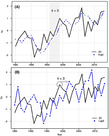
Figure 4. Illustration of the different types of time delays for surface temperature (SST) at k = 3: (A) moving average; (B) forward lag shift.

We first used a simple approach of incorporating delays by evaluating all combinations of predictors with the same type and length of delay (e.g., all predictors either Avgk or Lagk; Chen and Ware, 1999). Because pressures may manifest in the fish community biomass on different timescales (i.e., fishing acts immediately, environment generally takes longer), we repeated the analysis using strategically chosen delay types and lengths for each predictor.

Results

Zero Delay Models

The results for the three time periods using the ZD predictors are illustrated in Figure 5. Tables S1–S3 show which pressures were included in the top 50 models (i.e., top 10%) for each period. Inclusion of shellfish as a response in the After models had minimal effects, increasing the explanatory power only slightly, and highlighting the same number and most frequent indicators.

FIGURE 5

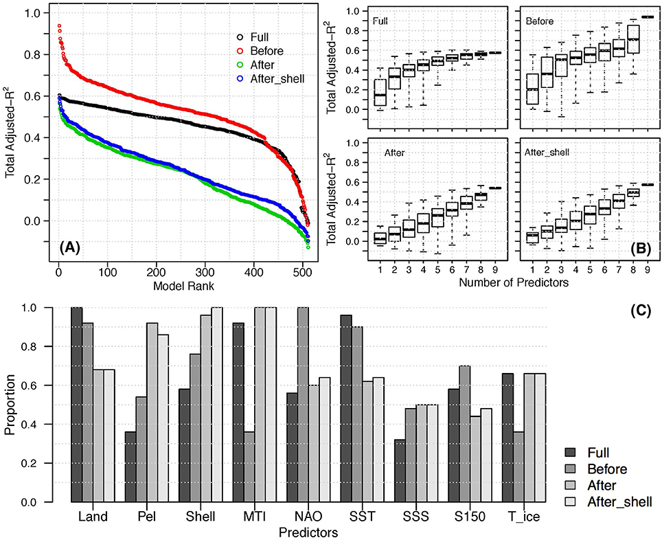
Figure 5. (A) Adjusted-${\text{R}}_{\text{Total}}^2$for zero-delay indicators of the three time periods; (B) The range of adjusted-${\text{R}}_{\text{Total}}^2$ for a given number of predictors for each time period; (C) Proportion of times each predictor appeared in the top 50 models of each time period. (“After_shell” indicates analysis that included the community shellfish biomass index as a response).

In general, the Before models had notably higher adjusted-${\text{R}}_{\text{Total}}^2$ than the After models, and the Full models had intermediate values (Figure 5). The best Before models had strikingly high explanatory power when compared to the other periods (adjusted-${\text{R}}_{\text{Total}}^2=$ 0.94 vs. ~0.60); however, lower-ranked (smaller adjusted-${\text{R}}_{\text{Total}}^2$) Before and Full models had similar explanatory power. The high adjusted-${\text{R}}_{\text{Total}}^2$ of the best Before models highlights the common signal among functional groups and the external pressures during this period. Most of the functional group biomasses decreased (Figure 2), as did total landings and MTI, while shellfish landings increased (Figure 3). The environmental pressures were more variable, but SST had a strong decreasing trend from the late 1980s until the early 1990s (Figure 3; Dempsey et al., 2017).

The adjusted-${\text{R}}_{\text{Total}}^2$ of the top 50 models and the corresponding adjusted-R² for each functional group further highlighted differences between the two periods (Figure 6). The high explanatory power for large benthivores and piscivores (average adjusted-R² of 0.95 and 0.91, respectively) contributed to the remarkably high overall explanatory power for the Before period. The adjusted-R² for medium and small benthivores was also notably higher than the adjusted-${\text{R}}_{\text{Total}}^2$ for this period, while planktivores and plank-piscivores had the lowest average explanatory power. In contrast, plank-piscivores and medium benthivores had the highest explanatory power for the After period. Piscivores and small benthivores, which were among the best predicted in the Before period, had the lowest average adjusted-R² for the top 50 After models.

FIGURE 6

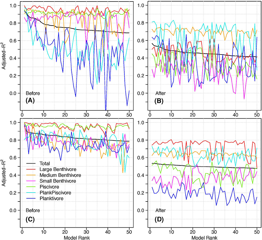
Figure 6. The adjusted-${\text{R}}_{\text{Total}}^2$ of the top 50 models and corresponding adjusted-R² of each functional group for (A) Before models, ZD predictors; (B) After models, ZD predictors; (C) Before models, Avg1 predictors; (D) After models, Avg1 predictors. The legend is the same for each panel.

There is a clear plateau in the overall explanatory power of the Full models, with the best set of three predictors (total landings, MTI and SST; see Table S1) having only a marginally different adjusted-${\text{R}}_{\text{Total}}^2$ than sets with more predictors (Figure 5B). Six predictors were used in the best model for the Full period, (adjusted-${\text{R}}_{\text{Total}}^2$ = 0.60), although all top 50 sets had adjusted-${\text{R}}_{\text{Total}}^2$ within 0.05 (sets of 3–9 predictors). In contrast, the Before models did not plateau, with the best set requiring all 9 predictors (adjusted-${\text{R}}_{\text{Total}}^2$ = 0.94). All of the top 50 Before models have higher explanatory power than the best Full and After models. The best After model used 8 predictors (adjusted-${\text{R}}_{\text{Total}}^2$ = 0.59 including shellfish as a response, and 0.56 excluding shellfish), although there were sets of 6, 7, and 9 predictors with similar explanatory power. The lower adjusted-${\text{R}}_{\text{Total}}^2$of the After (and Full) models suggests that there is at least one pressure not included here that could improve the explanatory power for these periods. In general, using less predictors in the Before and After models sacrificed more explanatory power than for the Full models. The range of adjusted-${\text{R}}_{\text{Total}}^2$ for a given number of predictors is generally smaller for the Full time series compared to the Before and After models (Figure 5B). For example, the range for 6-predictor Before models is over three times larger than that of 6-predictor Full time series models. This suggests that for the Full models, the number of predictors included is more important than which predictors are included. For the other two periods, a specific set of p predictors has high explanatory power, while other sets of p predictors do not.

Several predictors have much different inclusion frequencies Before and After the collapse, suggesting that different pressures were most influential in these two periods (Figure 5C). These differences are obscured by considering only the Full time series, underscoring the importance of selecting an ecologically coherent time frame for indicator analysis (Dempsey et al., 2017). As expected, the frequency of landings indicators reflects the change in target species after the collapse and subsequent groundfish moratoria. Total landings (which are highly correlated with groundfish landings; Dempsey et al., 2017), are more frequent in the Before models, while pelagic and shellfish landings are more frequent in the After models. The MTI was included in almost all of the Full and After models, but less than half of the Before models. This may be explained by the changes in fishing pressures after the collapse and moratoria. Before the collapse, MTI was highly correlated with the other fishing predictors because most of the landings were high trophic level species. After the collapse, MTI was not highly correlated with the other fishing predictors, indicating that it provides different information, which may be why it is included in so many of the best After models. The most notable differences in the environmental predictors were NAO and SST, which were included in all or most of the Before models, respectively, but in only about 60% of the After models. This suggests that environmental conditions were more influential Before the collapse, and/or that relationships between the fish functional groups and these specific environmental pressures were more linear before the collapse.

Delay Models

The above analysis showed that there are ecologic differences between the Before and After periods, and that the relationships for Full period do not represent either. As such, for the delay analysis we focussed on the two periods separately. In general, the moving average predictors improved the explanatory power more than the lag predictors (Figure 7). The delay with the highest explanatory power for both periods was Avg1, a 2-year moving average including the current year, i and year i−1. The Before Avg1 models were marginally better than the top 10 ZD models, and were notably better for most of the remaining models. The other Before moving average models had lower or marginally higher explanatory power than ZD models (until worse ranks). The After Avg1 models were marginally different than the top 25 ZD models, and notably better for the rest of the models.

FIGURE 7

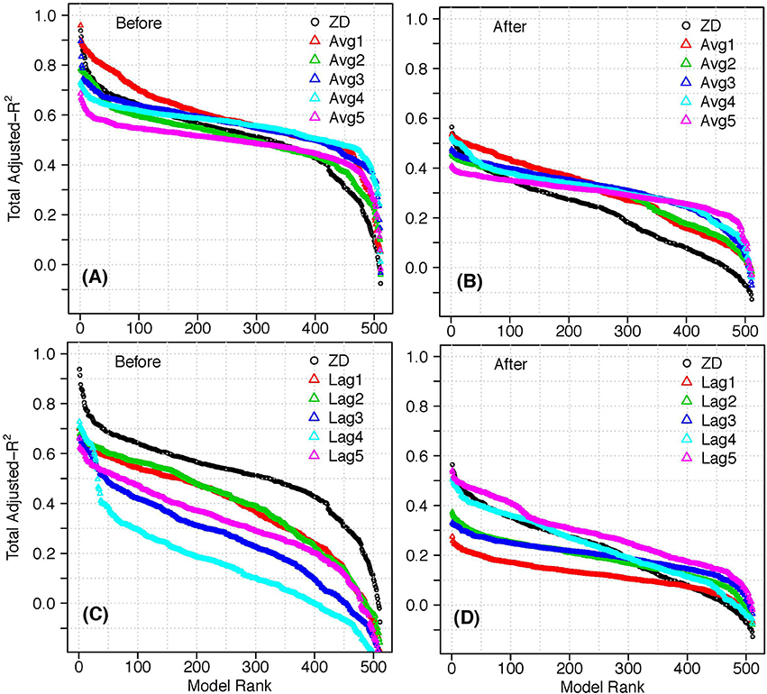
Figure 7. Adjusted-${\text{R}}_{\text{Total}}^2$ in decreasing rank for models using predictors with time delays: (A) Before models, moving average predictors; (B) After models, moving average predictors; (C) Before models, lag predictors; (D) After models, lag predictors.

We investigated how delays affect the explanatory power of individual functional groups using the Avg1 predictors (i.e., the best delay type and length). In general, the adjusted-R² for each functional group increased for the Avg1 predictors compared to the ZD predictors (Figure 6). The most notable improvements were for plank-piscivores and planktivores in the Before period, and large benthivores for the After (adjusted-R² increased by ~0.30 for each). The explanatory power for several functional groups decreased with the Avg1 predictors (small and medium benthivores Before; small benthivores, plank-piscivores, and planktivores After), but these changes were minor when compared to the improvements of the other groups. Another striking feature of Figure 6 is the reduced variance in the adjusted-R² for each functional group (except large benthivores) for the Avg1 predictors. This is most noticeable for the adjusted-R² of the planktivores in the Before period, which had a standard deviation of 0.29 with ZD predictors vs. 0.08 with Avg1 predictors.

The results of the lag analysis were less consistent between the two periods. All the models with lag predictors for the Before period had notably lower explanatory power than with ZD predictors. This could suggest that the major pressures on the fish community during this time were related to fisheries removals, which have immediate primary effects on the ecosystem. In contrast, the After Lag4 models had similar explanatory power as the ZD models, while the Lag5 predictors were similar or marginally better for the top 50 models, and notably better for some models at worse ranks. This suggests that the fish community could also be experiencing indirect effects of fishing (e.g., Daan et al., 2005; Koen-Alonso et al., 2010), or environmental effects that require time to manifest in the system.

For most delays, subsets of the predictors had similar or higher explanatory power than the full suite (Figure 8; Supplementary Figures). In general, the range of adjusted-${\text{R}}_{\text{Total}}^2$ for a given number of predictors was larger for the Before models than the After, suggesting that which pressures included in the subset was more important Before, and the number of pressures included was more important After. For all delays (except Before Avg1 and Avg3), the adjusted-${\text{R}}_{\text{Total}}^2$ plateaued or decreased after a certain number of predictors were used.

FIGURE 8

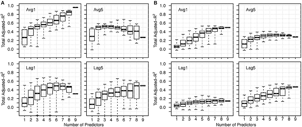
Figure 8. The range of adjusted-${\text{R}}_{\text{Total}}^2$ for a given number of predictors all delayed by k for moving average and lag predictors (A) Before models; (B) After models. Select k are shown here; see Figures S1 and S2 for all k.

There are some notable differences in the patterns of most frequent predictors between the two delay types (Figure 9). In the Before models, total landings were most frequent at ZD, which was expected because the ecosystem was heavily exploited during this period, especially for groundfish (represented by total landings, Dempsey et al., 2017). Pelagic and shellfish landings were also expected to be most frequent at ZD, but were more frequent at higher delays, which suggests indirect effects of fishing. Shellfish landings were included in about 80% of the ZD and Avg2 models, and almost all the Lag1, Lag2, and Lag3 models. This was unexpected because there were limited commercial shellfish landings at this time, and because shellfish was not included as a functional group response. One possible interpretation is that because shellfish landings were increasing approximately linearly with time (Figure 3), they were highly negatively correlated with the declines in the other functional groups, and therefore contributed to explaining variance in the responses. Both MTI and NAO were included in almost all of the top Lag3 models, but only about 60% of the Avg3 models. In contrast, SST was included in all of the Avg2 and Avg3 models, but less than half of the lag models at these same k. S150 and Time_Ice were also included in notably more Avg models than Lag models.

FIGURE 9

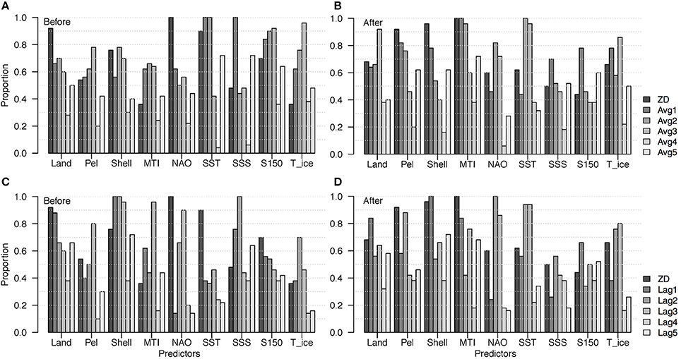
Figure 9. Proportion of times each predictor appeared in the top 50 models of the Before and After models for each delay type and length: (A) Before models, moving average predictors; (B) After models, moving average predictors; (C) Before models, lag predictors; (D) After models, lag predictors.

In the After models, total landings were more frequent at delays (Avg3 and Lag1; Figure 9), which could indicate delayed effects of fishing on the fish community structure. Pelagic landings were most frequent at ZD (closely followed by Lag2), and shellfish landings were included in almost all the ZD and Lag1 models, which is curious because the community shellfish index was not included as a response for that analysis. MTI was included in most of the ZD, Avg1, and Avg2 models. NAO was included in all the Lag2 models, but only about 80% of the Avg models, while SST was most frequent at delays of 2 and 3 years for both delay types. SSS was not particularly frequent in any of the lag models, but was included in about 70% of of Avg1. S150 and Time_Ice were most frequent at the same k for both delay types (k = 1 and k = 3, respectively).

We repeated the analysis using specific delays for each predictor (“Mix” models) based on the idea that fishing pressures have shorter time delays, while environmental pressures take longer to manifest in the fish community. None of the combinations of delay types and lengths we tested had notably higher explanatory power than the best ZD and Avg1 Before models (not shown). In contrast, several combinations of mixed delay pressures were notably better than the best After models (e.g., Mix1 and Mix2, Figure 10). Mix1 and Mix2 both had shorter time delays (ZD, k = 1) for most of the fishing pressures and longer delays (k = 2+) for most of the environmental pressures. The top 50 Mix1 models included sets of 5–9 predictors, with total landings, MTI, and SST being the most frequent. The best set used 7 predictors, but there were other sets of 7–9 with only marginally different explanatory power. The top 50 Mix2 models included sets of 4–9 predictors, with pelagic landings, NAO, SST, and Time_Ice the most frequent. The best Mix2 set used 6 predictors, and there were other sets of 5–8 with only marginally different explanatory power. The delays for Mix3 were chosen to provide a counter-example where all pressures have longer delays except NAO, which was assigned ZD. As expected, Mix3 was notably worse than the After ZD models, and NAO was not present in most of these “best” models.

FIGURE 10

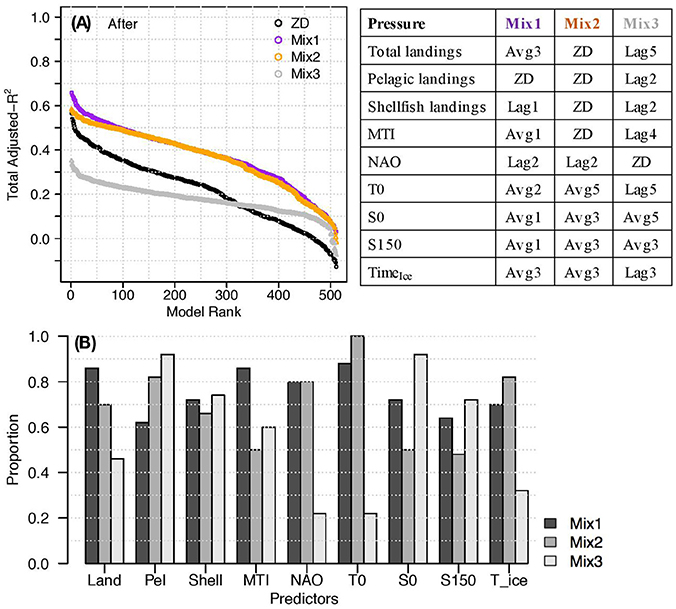
Figure 10. (A) Adjusted-${\text{R}}_{\text{Total}}^2$ in decreasing rank for After models using predictors with mixed time delays; (B) Proportion of times each predictor appeared in the top 50 models for each set of After mix delays. Refer to table legend for type and length of delay used for each predictor.

Discussion

Our analysis adds to the literature demonstrating that there is no single type of pressure driving fish community dynamics on the Newfoundland shelf (e.g., Mann and Drinkwater, 1994; Devine et al., 2007; Koen-Alonso et al., 2010). In this study, both fishing and environmental indicators were included in nearly all the top models for all types and lengths of time delays (exceptions are five After models with adjusted-${\text{R}}_{\text{Total}}^2\le$ 0.40), which highlights that managers in this area should factor both types of pressures into their decisions. The dominant pressures Before the collapse of fish biomass (i.e., those that caused the collapse) in the Northwest Atlantic have been the subject of debate, especially for commercially important species such as Atlantic cod. Some authors conclude that fishing mortality was the sole major cause of the collapse (e.g., Myers et al., 1996, 1997), even though non-commercial species were also impacted (e.g., Gomes et al., 1995 for Division 2J3KL, NAFO, 2010b for Divisions 2K3KL and 3LNO). Others assert the poor environmental conditions were an important driving pressure (e.g., Parsons and Lear, 2001; Rothschild, 2007; Halliday and Pinhorn, 2009), pointing out for example that the community recovered from a similar collapse in the 1970s, when fishing pressure was high, but environmental conditions were more favorable than the early 1990s. Our analysis supports a broader argument that the combination of these two drivers (high fishing and poor environment) were necessary for the extensive and widespread changes that occurred (e.g., Rose, 2004; Devine et al., 2007; Koen-Alonso et al., 2010). Specifically, total landings (here also a proxy for groundfish landings), NAO and SST were the most frequent pressures included the best (top 50) Before models. The best 1-predictor model was total landings (adjusted-${\text{R}}_{\text{Total}}^2$ = 0.55), while the best 2-predictor model included total landings and NAO (adjusted-${\text{R}}_{\text{Total}}^2$ = 0.63), and including SST further improved the explanatory power (adjusted-${\text{R}}_{\text{Total}}^2$ = 0.67). The inclusion of both NAO and SST speaks to the importance of both basin and local environmental effects on the ecosystem, further strengthening the need to have regional information to understand and predict changes in the fish community.

Our analysis shows that there was a shift in which fishing and environmental pressures were most directly related to the fish community structure Before and After the collapse. The environment can clearly influence fish community dynamics on the Grand Bank, but the most frequently included pressures in the ZD After models are pelagic and shellfish landings and MTI. This set of three pressures has notably higher overall explanatory power Before the collapse; however, its adjusted-${\text{R}}_{\text{Total}}^2$ represents a higher percentage of the maximum explanatory power for the After period. This suggests that the remaining pressures (e.g., environment) add relatively less predictive information in the After models. This shift reflects the changes in target species after the groundfish moratoria, although it is somewhat surprising that shellfish landings were included in all but two top models, because the community shellfish biomass was not included as a response. Shellfish landings consist mainly of snow crab and Pandalus shrimp, while pelagic landings are mainly capelin. Shrimp and capelin are considered important forage species on the Grand Bank (DFO, 2015a,b), and are managed conservatively (for example there is capelin moratorium in 3NO); however, our analysis suggests landings of these species are impacting the ecosystem. Shellfish landings increased overall in the After period (despite a slight decrease in the last several years), and are negatively correlated with the biomass indices of small benthivores, piscivores, and plank-piscivores, suggesting that they are hindering the recovery of these functional groups. The question remains whether this is indicative of a causal relationship, or is only correlative. One potential mechanistic explanation is given by Koen-Alonso et al. (2010), who speculated that fishing may be reducing food availability for key species on the Grand Banks, and thus hindering their recovery. Another hypothesis is that there are secondary effects on the fish community from shrimp beam trawls. These trawls are considered to have low bycatch rates (for commercial species; NAFO, 2014), but they could be negatively impacting the habitat of other species in the community.

Another striking difference between the two periods is the remarkably high explanatory power of the best Before models compared to the best After models (Figure 5) for any time delay (type or length) or number of predictors. We can speculate that the reasons for this relate to changes in relationships among and within the pressures and responses. For example, there was a strong signal in the responses Before the collapse. The biomasses of many functional groups were relatively highly correlated (Dempsey et al., 2017), such that any set of predictors with high explanatory power for one particular group was also high for several of the others (e.g., small, medium, and large benthivores and piscivores; Figure 6). The weaker signal After the collapse means prediction of all six functional groups may require a broader spectrum of pressures.

We showed the pressures that were driving changes Before the collapse are no longer as influential After, and the relatively lower adjusted-${\text{R}}_{\text{Total}}^2$ suggests that there may be pressures missing from the After models. Bottom up pressure indicators such as primary production and trophic transfer efficiencies were not included here because there was no suitable data for the required time frame. Our models include the timing of the sea ice melt as a proxy for the timing of phytoplankton spring bloom, but other characteristics of the bloom (e.g., duration and magnitude), or lower trophic level energy transfer may prove better predictors for this period through some mechanism not identified here. Other missing pressures are measures of predation by sea birds and marine mammals that could exert a top-down influence on the fish community. For example, harp seals migrate from the Arctic to northern Newfoundland in the Fall, and prey predominantly on capelin, but also eat other species (e.g., Atlantic herring, Arctic cod, shrimp, and Atlantic cod; Stenson, 2013). The Northwest Atlantic harp seal population has been increasing rapidly since the 1980s (Hammill et al., 2011), and some authors suggest that seal predation has supressed the recovery of fish species on the Newfoundland-Labrador shelf (e.g. Bundy, 2001; Devine et al., 2007). One type of human-related pressure specific to the After period that wasn't considered here is oil production. While oil exploration has occurred on the Grand Banks since the 1960s, active platforms have only been producing oil since 1997. Related pressures could include chemical pollution from regular discharge or accidental spills (Templeman, 2010), which can be especially harmful to early life stages, and can disrupt development, growth, and reproductive rates (etc., see JWL, 2007 and references therein). These pressures were not included here because we did not expect them to significantly influence the Grand Bank fish community; however, our analyses suggest that future investigations into these pressures are warranted.

Finally, non-linearity in the relationships between pressures and responses may have a stronger influence during the After period, through some unidentified mechanism. Predator-prey relationships, population dynamics, environmental changes, and human impacts can all result in non-linearity in marine ecosystems (Liu et al., 2014). Given the significant changes in the fish community structure and related pressures, we can speculate that the relationships among them could be less linear After the collapse, resulting in lower explanatory power because RDA is based on linear regression. This could be tested by comparing this analysis to results from a non-linear model such as neural networks or generalized additive models. These flexible models don't require the user to specify the forms of the relationships between predictors and responses, which affords a potential advantage of being able to capture the nonlinearity when the mechanistic forms of these relationships are unknown.

Our analysis showed that incorporating delays can improve explanatory power, but that the type and length of delay should be carefully considered. In general, moving average predictors had higher explanatory power than lagged predictors for both periods. Since the moving averages incorporate the trend in the predictors, causing the responses to change gradually over time (see Figure A1 in Gentleman and Neuheimer, 2008), our results suggest that trends in these pressures are influencing the fish community. For the models with the same delay type and length for each predictor, Avg1 was the best, notably improving the explanatory power compared to ZD for both periods. Avg1 also increased the explanatory power and reduced the variability in the adjusted-R² for most of the individual functional groups (Figure 6). Other delays, particularly those with lagged predictors, had notably worse explanatory power than ZD. While some of the improved fit of the moving averages may be an artifact of smoothing, our results still strongly suggest that the rates of change are useful for predicting.

Our examination of Mixed delays illustrated that the explanatory power of the Avg1 After models can be further improved by considering simple relationships when choosing the delays for each predictor (Figure 10). This suggests that including the different timescales of influence for the pressures is important for this period, and could improve the ability to forecast changes in the fish community. Even longer time delays could be beneficial because changes in some pressures may take more than 5 years to manifest in the fish community. For example, Daan et al. (2005) and Greenstreet et al. (2011) found that secondary effects of fishing could impact different size-based metrics of the fish community in the North Sea after lags of 6–12 and 12–20 years, respectively. However, while we showed that different mixed delays among the predictor set resulted in similar overall explanatory power, we also showed it could be worse. We therefore recommend that future investigations into suitable delays—and their mechanisms—should come from analysis of mechanistic models.

For all three periods (Full, Before, and After) and delay types and lengths, there was no one set of pressures that “best” predicted fish community status. Rather there was a range of sets, differing in number and type of indicators that had similar explanatory power (see Tables S1–S5). For example, there are two sets of 6-pressure Avg1 After models with only marginally different explanatory power; however, one includes two fishing indicators (pelagic landings and MTI) and four environmental indicators (all except S150; adjusted-${\text{R}}_{\text{Total}}^2$ = 0.68), while the other includes all four fishing and two environmental (S150 and Time_Ice; adjusted-${\text{R}}_{\text{Total}}^2$ = 0.70). In many cases the same base indicators were used in most or all of the top sets (Figure 5C; e.g., for ZD After: pelagic and shellfish landings and MTI), while other pressures improved the explanatory power by adding additional information. This is not to say that any set of nine pressures would have high explanatory power—recall that we curated these pressures because we expected them to have measurable impacts on the Grand Bank fish community. The point here is that pressure sets with similar predictive power may be comprised of different types of strategically selected data. This suggests that various direct effects of pressures on fish and lower trophic level production have spread throughout the community such that changes in fish functional group biomass can be directly predicted from different pressures. Therefore, if there was a lack of one type of pressure data, it may be possible to replace it with another type without compromising explanatory power. Furthermore, using a suite of models to predict future changes can provide a measure of uncertainty, much like the model ensembles used to forecast climate changes and associated impacts by the Intergovernmental Panel on Climate Change (Kirtman et al., 2013).

Here we provided one case study of how RDA can be applied to learn about the Grand Bank ecosystem. Ultimately the best predictor set(s) for the Grand Bank and other ecosystems would depend on a number of considerations, including the final application of the model. Other considerations may include the responses of interest (i.e., if structure of the fish community were expanded to also consider length and/or biodiversity measures), the explanatory power for the individual responses (Figure 6), data availability (e.g., types of indicators and length of time series), and costs of monitoring (e.g., data collection, database entry, analysis). As well as potentially varying with application-specific criteria, best sets will likely be ecosystem-specific, and depend on the unique combination of exploitation history, oceanographic conditions, and ecological interactions. Finally, because ecosystems are dynamic and the types and intensity of pressures may change over time, the best predictor sets may differ for different time periods of the same ecosystem. Scientists and managers should be aware of this, and watch for declines in the ability of these sets to predict changes in the ecosystem. Here we offer a statistical approach that can be used with various types of data, and is suggestive of being easily calibrated to different systems. This could serve as a useful complementary tool to help design modeling studies, plan field programs, and direct monitoring efforts. The synergistic use of statistical and mechanistic models to help guide identification of the most informative pressures, their most influential time delays, and their mechanisms are important future research directions that could improve ability to forecast changes in the fish community, and implement appropriate management measures.

Author Contributions

DD and WG conceived of and designed the analysis. DD interpreted the results and drafted the manuscript. All authors provided critical input, and gave final approval of the version to be published.

Funding

DFO Ecosystem Research Initiative for the Newfoundland and Labrador Region (ERI-NEREUS), DFO International Governance Strategy (IGS), and DFO Strategic Program for Ecosystem-based Research and Advice (SPERA) programs provided logistical and financial support for this work. PP and MK-A were funded partly by DFO's Fisheries Science & Ecosystem Research Program (FSERP). WG and DD were supported by the Natural Science and Engineering Research Council of Canada.

Conflict of Interest Statement

The authors declare that the research was conducted in the absence of any commercial or financial relationships that could be construed as a potential conflict of interest.

The handling Editor declared a past co-authorship with one of the authors DD.

Supplementary Material

The Supplementary Material for this article can be found online at: https://www.frontiersin.org/articles/10.3389/fmars.2018.00037/full#supplementary-material

References

Atkinson, D. B. (1994). Some observations on the biomass and abundance of fish captured during stratified- random bottom trawl surveys in NAFO divisions 2J and 3KL, Autumn 1981 – 1991. NAFO Sci. 21, 43–66.

Belgrano, A., and Fowler, C. W. (eds.) (2011). Ecosystem Based Management for Marine Fisheries. New York, NY: Cambridge Unviersity Press.

Google Scholar

Bundy, A. (2001). Fishing on ecosystems: the interplay of fishing and predation in Newfoundland and Labrador. Can. J. Fish. Aquat. Sci. 58, 1153–1167. doi: 10.1139/f01-063

CrossRef Full Text | Google Scholar

Buren, A. D., Koen-Alonso, M., Pepin, P., Mowbray, F., Nakashima, B., Stenson, G., et al. (2014). Bottom-up regulation of capelin, a keystone forage species. PLoS ONE 9:e87589. doi: 10.1371/journal.pone.0087589

PubMed Abstract | CrossRef Full Text | Google Scholar

Caddy, J. F., and Garibaldi, L. (2000). Apparent changes in the trophic composition of world marine harvests: the perspective from the FAO capture database. Ocean Coast. Manag. 43, 615–655. doi: 10.1016/S0964-5691(00)00052-1

CrossRef Full Text | Google Scholar

Chen, D. G., and Ware, D. M. (1999). A neural network model for forecasting fish stock recruitment. Can. J. Fish. Aquat. Sci. 56, 2385–2396. doi: 10.1139/f99-178

CrossRef Full Text | Google Scholar

Daan, N., Gislason, H., Pope, J. G., and Rice, J. C. (2005). Changes in the North Sea fish community: evidence of indirect effects of fishing? ICES J. Mar. Sci. 62, 177–188. doi: 10.1016/j.icesjms.2004.08.020

CrossRef Full Text | Google Scholar

Dempsey, D. P., Koen-Alonso, M., Gentleman, W. C., and Pepin, P. (2017). Compilation and discussion of driver, pressure, and state indicators for the Grand Bank ecosystem, Northwest Atlantic. Ecol. Indic. 75, 331–339. doi: 10.1016/j.ecolind.2016.12.011

CrossRef Full Text | Google Scholar

Department of Fisheries and Aquaculture (2014). Seafood Industry Year in Review - 2013. Available online at: http://www.fishaq.gov.nl.ca/publications/pdf/SYIR_2013.pdf

Devine, J. A., Zuur, A. F., Ieno, E. N., and Smith, G. M. (2007). “Common trends in demersal communities on the Newfoundland-Labrador shelf,” in Analysing Ecological Data, eds A. F. Zuur, E. N. Ieno, and G. M. Smith (New York, NY: Springer), 672.

Google Scholar

DFO (2007). A New Ecosystem Science Framework in Support of Integrated Management. Available online at: http://www.dfo-mpo.gc.ca/science/publications/ecosystem/index-eng.htm

DFO (2009). Sustainable Fisheries Framework. Available online at: http://www.dfo-mpo.gc.ca/reports-rapports/regs/sff-cpd/overview-cadre-eng.htm (Accessed on July 20, 2017).

DFO (2014). Corporation Designation Policy and Procedures. Available online at: http://www.dfo-mpo.gc.ca/fm-gp/sdc-cps/nir-nei/obs-dpp-eng.htm (Accessed July 20, 2017).

DFO (2015a). Assessment of Northern Shrimp (Pandalus borealis) in Shrimp Fishing Areas 4-6 (NAFO Divisions 2G-3K) and of Striped Shrimp (Pandalus montagui) in Shrimp Fishing Area 4 (NAFO Division 2G). 2015/018.

DFO (2015b). Assessment of Capelin in Subarea 2 and Divisions 3KL in 2015.

DFO (2016). The National Vessel Monitoring System. Available online at: http://www.nfl.dfo-mpo.gc.ca/e0010178

Elliott, M. (2011). Marine science and management means tackling exogenic unmanaged pressures and endogenic managed pressures – a numbered guide. Mar. Pollut. Bull. 62, 651–655. doi: 10.1016/j.marpolbul.2010.11.033

PubMed Abstract | CrossRef Full Text

Fogarty, M. J. (2014). The art of ecosystem-based fishery management. Can. J. Fish. Aquat. Sci. 71, 479–490. doi: 10.1139/cjfas-2013-0203

CrossRef Full Text

Gari, S. R., Newton, A., and Icely, J. D. (2015). A review of the application and evolution of the DPSIR framework with an emphasis on coastal social-ecological systems. Ocean Coast. Manag. 103, 63–77. doi: 10.1016/j.ocecoaman.2014.11.013

CrossRef Full Text | Google Scholar

Gentleman, W. C., and Neuheimer, A. B. (2008). Functional responses and ecosystem dynamics : how clearance rates explain the influence of satiation, food-limitation and acclimation. J. Plankton Res. 30, 1215–1231. doi: 10.1093/plankt/fbn078

CrossRef Full Text | Google Scholar

Gomes, M. C., Haedrich, R. L., and Villagarcia, M. G. (1995). Gomes_1995.pdf. Fish. Oceanogr. 4, 85–101. doi: 10.1111/j.1365-2419.1995.tb00065.x

CrossRef Full Text

Greenstreet, S. P. R., Rogers, S. I., Rice, J. C., Piet, G. J., Guirey, E. J., Fraser, H. M., et al. (2011). Development of the EcoQO for the North Sea fish community. ICES J. Mar. Sci. 68, 1–11. doi: 10.1093/icesjms/fsq156

CrossRef Full Text | Google Scholar

Gröger, J. P., and Fogarty, M. J. (2011). Broad-scale climate influences on cod (Gadus morhua) recruitment on Georges Bank. ICES J. Mar. Sci. 68, 592–602. doi: 10.1093/icesjms/fsq196

CrossRef Full Text | Google Scholar

Halliday, R. G., and Pinhorn, A. T. (2009). The roles of fishing and environmental change in the decline of Northwest Atlantic groundfish populations in the early 1990s. Fish. Res. 97, 163–182. doi: 10.1016/j.fishres.2009.02.004

CrossRef Full Text | Google Scholar

Hamilton, L. C., and Butler, M. J. (2001). Outport adaptations: social indicators through Newfoundland's Cod crisis. Hum. Ecol. Rev. 8, 1–11. Available online at: https://scholars.unh.edu/soc_facpub/169/

Google Scholar

Hammill, M. O., Stenson, G. B., Doniol-Valcroze, T., and Mosnier, A. (2011). Northwest Atlantic Harp Seals Population Trends, 1952-2012. DFO Canadian Science Advisory SecretariatScience Advisory Report 2011/070.

Heymans, J. J., Coll, M., Link, J. S., Mackinson, S., Steenbeek, J., Walters, C., et al. (2016). Best practice in Ecopath with Ecosim food-web models for ecosystem-based management. Ecol. Modell. 331, 173–184. doi: 10.1016/j.ecolmodel.2015.12.007

CrossRef Full Text | Google Scholar

Hurrell, J. W. (1995). Decadal trends in the North Atlantic Oscillation: regional temperatures and precipitation. Science 269, 676–679. doi: 10.1126/science.269.5224.676

PubMed Abstract | CrossRef Full Text | Google Scholar

Jennings, S. (2005). Indicators to support an ecosystem approach to fisheries. Fish Fish. 6, 212–232. doi: 10.1111/j.1467-2979.2005.00189.x

CrossRef Full Text | Google Scholar

JWL (2007). “Chapter 5: potential environmental effects from exploration and production activities,” Sydney Basin Strategic Environmental Assessment: Final Report. Prepared for CNLOPB.

Kirtman, B., Power, S., Adedoyin, J., Boer, G., Bojariu, R., Camilloni, F., et al. (2013). “Near-term climate change: projections and predictability,” in Climate Change 2013: The Physcial Science Basis, eds T. Stocker, D. Qin, G.-K. Plattner, M. Tignor, S. Allen, J. Boschung, et al. (New York, NY; Cambridge: Cambridge Unviersity Press), 959–961.

Google Scholar

Koen-Alonso, M., Pepin, P., and Mowbray, F. (2010). Exploring the Role of Environmental and Anthropogenic Drivers in the Trajectories of Core Fish Species of the Newfoundland-Labrador Marine Community.

Large, S. I., Fay, G., Friedland, K. D., and Link, J. S. (2015). Quantifying patterns of change in marine ecosystem response to multiple pressures. PLoS ONE 10:e0119922. doi: 10.1371/journal.pone.0119922

PubMed Abstract | CrossRef Full Text | Google Scholar

Larkin, P. A. (1996). Concepts and issues in marine ecosystem management. Rev. Fish Biol. Fish. 6, 139–164. doi: 10.1007/BF00182341

CrossRef Full Text | Google Scholar

Legendre, P., and Legendre, L. (2012). Numerical Ecology, 3rd Edn. Amsterdam: Elsevier, B.V.

Google Scholar

Legendre, P., Oksanen, J., and ter Braak, C. J. F. (2011). Testing the significance of canonical axes in redundancy analysis. Methods Ecol. Evol. 2, 269–277. doi: 10.1111/j.2041-210X.2010.00078.x

CrossRef Full Text | Google Scholar

Lilly, G. R., Parsons, D. G., and Kulka, D. W. (2000). Was the increase in shrimp biomass on the northeast newfoundland shelf a consequence of a release in predation pressure from cod? J. Northwest Atl. Fish. Sci. 27, 45–61. doi: 10.2960/J.v27.a5

CrossRef Full Text | Google Scholar

Link, J. S., Fulton, E. A., and Gamble, R. J. (2010a). Progress in Oceanography The northeast US application of ATLANTIS : a full system model exploring marine ecosystem dynamics in a living marine resource management context. Prog. Oceanogr. 87, 214–234. doi: 10.1016/j.pocean.2010.09.020

CrossRef Full Text | Google Scholar

Link, J. S., Yemane, D., Shannon, L. J., Coll, M., Shin, Y. J., Hill, L., et al. (2010b). Relating marine ecosystem indicators to shing and environmental drivers: an elucidation of contrasting responses. ICES J. Mar. Sci. 67, 787–795. doi: 10.1093/icesjms/fsp258

CrossRef Full Text | Google Scholar

Liu, H., Fogarty, M. J., Hare, J. A., Hsieh, C., Glaser, S. M., Ye, H., et al. (2014). Modeling dynamic interactions and coherence between marine zooplankton and fishes linked to environmental. J. Mar. Syst. 131, 120–129. doi: 10.1016/j.jmarsys.2013.12.003

CrossRef Full Text | Google Scholar

Mann, K. H., and Drinkwater, K. F. (1994). Environmental influences on fish and shellfish production in the Northwest Atlantic. Environ. Rev. 2, 16–32. doi: 10.1139/a94-002

CrossRef Full Text | Google Scholar

McCallum, B. R., and Walsh, S. J. (1997). Groundfish survey trawls used at the Northwest Atlantic fisheries centre, 1971 to present. NAFO Sci. Counc. Stud. 29, 93–104.

Misund, O. A., and Skjoldal, H. R. (2005). Implementing the ecosystem approach: experiences from the North Sea, ICES, and the Institute of Marine Research, Norway. Mar. Ecol. Prog. Ser. 300, 260–265. doi: 10.3354/meps300260

CrossRef Full Text | Google Scholar

Myers, R. A., Hutchings, J. A., and Barrowman, N. J. (1996). Hypotheses for the decline of cod in the North Atlantic. Mar. Ecol. Prog. Ser. 138, 293–308. doi: 10.3354/meps138293

CrossRef Full Text | Google Scholar

Myers, R. A., Hutchings, J. A., and Barrowman, N. J. (1997). Why do fish stocks collapse? The example of cod in Atlantic Canada. Ecol. Appl. 7, 91–106. doi: 10.1890/1051-0761(1997)007[0091:WDFSCT]2.0.CO;2

CrossRef Full Text | Google Scholar

NAFO (2010a). Part B: Scientific Council Meeting, 3-16 June 2010.

NAFO (2010b). Report of the NAFO Scientific Council Working Group on Ecosystem Approaches to Fisheries Management (WGEAFM). NAFO SCS Doc. 10/ 19. Serial No. N5815.

NAFO (2014). Report of the 7th Meeting of the NAFO Scientific Council (SC) Working Group on Ecosystem Science and Assessment (WGESA) [Formerly SC WGEAFM]. NAFO SCS Doc. 14/023 Serial No. N6410.

NAFO (2017). Northwest Atlantic Fisheries Organization Conservation and Enforcement Measures. NAFO FC Doc. 17-01. Serial No. N6638.

Oceans Act (1996). Available online at: http://laws-lois.justice.gc.ca/eng/acts/O-2.4/

Ojaveer, H., and Eero, M. (2011). Methodological challenges in assessing the environmental status of a marine ecosystem: case study of the Baltic Sea. PLoS ONE 6:e19231. doi: 10.1371/journal.pone.0019231

PubMed Abstract | CrossRef Full Text | Google Scholar

Parsons, L. S., and Lear, W. H. (2001). Climate variability and marine ecosystem impacts : a North Atlantic perspective. Progr. Oceanogr. 49, 167–188. doi: 10.1016/S0079-6611(01)00021-0

CrossRef Full Text | Google Scholar

Pedersen, E. J., Thompson, P. L., Ball, A. R., Fortin, M.-J., Gouhier, T. C., Link, H., et al. (2017). Signatures of the collapse and incipient recovery of an overexploited marine ecosystem. R. Soc. Open Sci. 4:170215. doi: 10.1098/rsos.170215

PubMed Abstract | CrossRef Full Text | Google Scholar

Petrie, B. (2007). Does the North Atlantic oscillation affect hydrographic properties on the Canadian Atlantic continental shelf? Atmos. Ocean 45, 141–151. doi: 10.3137/ao.450302

CrossRef Full Text | Google Scholar

Rice, J. C., and Rochet, M.-J. (2005). A framework for selecting a suite of indicators for fisheries management. ICES J. Mar. Sci. 527, 516–527. doi: 10.1016/j.icesjms.2005.01.003

CrossRef Full Text | Google Scholar

Rice, J. (2003). Environmental health indicators. Ocean Coast. Manag. 46, 235–259. doi: 10.1016/S0964-5691(03)00006-1

CrossRef Full Text | Google Scholar

Rose, G. A. (2004). Reconciling overfishing and climate change with stock dynamics of Atlantic cod (Gadus morhua) over 500 years. Can. J. Fish. Aquat. Sci. 61, 1553–1557. doi: 10.1139/f04-173

CrossRef Full Text | Google Scholar

Rose, G. A. (2007). Cod: The Ecological History of the North Atlantic Fisheries. St. John's, NL: Breakwater Books.

Google Scholar

Rothschild, B. J. (2007). Coherence of Atlantic cod stock dynamics in the Northwest Atlantic Ocean. Trans. Am. Fish. Soc. 136, 858–874. doi: 10.1577/T06-213.1

CrossRef Full Text | Google Scholar

Schrank, W. E. (2005). The Newfoundland fishery: ten years after the moratorium. Mar. Policy 29, 407–420. doi: 10.1016/j.marpol.2004.06.005

CrossRef Full Text | Google Scholar

Shannon, L. J., Coll, M., Yemane, D., Jouffre, D., Neira, S., Bertrand, A., et al. (2010). Comparing data-based indicators across upwelling and comparable systems for communicating ecosystem states and trends. ICES J. Mar. Sci. 67, 807–832. doi: 10.1093/icesjms/fsp270

CrossRef Full Text | Google Scholar

Shin, Y.-J., Shannon, L. J., Bundy, A., Coll, M., Aydin, K., Bez, N., et al. (2010). Using indicators for evaluating, comparing, and communicating the ecological status of exploited marine ecosystems. 2. Setting the scene. ICES J. Mar. Sci. 67, 692–716. doi: 10.1093/icesjms/fsp294

CrossRef Full Text | Google Scholar

Stenson, G. B. (2013). Estimating consumption of prey by Harp Seals (Pagophilus groenlandicus) in NAFO Divisions 2J3KL. DFO Can. Sci. Advis. Sec. Res. Doc. 2012/156. iii + 26 p. (Errata: October 2015)

Templeman, N. D. (2010). Ecosystem Status and Trends Report for the Newfoundland and Labrador Shelf.

Whittingham, M. J., Stephens, P. A., Bradbury, R. B., and Freckleton, R. P. (2006). Why do we still use stepwise modelling in ecology and behaviour? J. Anim. Ecol. 75, 1182–1189. doi: 10.1111/j.1365-2656.2006.01141.x

PubMed Abstract | CrossRef Full Text | Google Scholar

Wu, Y., Peterson, I. K., Tang, C. C. L., Platt, T., Sathyendranath, S., and Fuentas-Yaco, C. (2007). The impact of sea ice on the initiation of the spring bloom on the Newfoundland and Labrador Shelves. J. Plankton Res. 29, 509–514. doi: 10.1093/plankt/fbm035

CrossRef Full Text | Google Scholar