A Package for Measuring Emergence, Self-organization, and Complexity Based on Shannon Entropy

1. Description

Complexity has generated interest in recent years (Bar-Yam, 1997; Mitchell, 2009; Haken and Portugali, 2017). A complex system can be understood as one composed by many elements, which acquire functional/spatial/temporal structures without a priori specifications (Haken and Portugali, 2017). It has been studied in several disciplines, as one can try to measure the complexity of almost any phenomenon (Lopez-Ruiz et al., 1995; Bandt and Pompe, 2002; Prokopenko et al., 2009; Lizier, 2014; Soler-Toscano et al., 2014; Haken and Portugali, 2017). Thus, there exist a broad variety of measures of complexity where Shannon’s entropy and its generalizations have played a crucial role (Haken and Portugali, 2017). For instance, permutation entropy have been proposed for analyzing the complexity of time series in terms of its periodicity/chaoticity/randomness (Bandt and Pompe, 2002), whereas the LMC Complexity describe it in terms of equilibrium and disequilibrium (Lopez-Ruiz et al., 1995). Nevertheless, it should be noted that all measures of complexity have limits (Zenil and Kiani, 2016). Thus, it is important to promote the quantitative study of complexity through mathematical frameworks to enhance the exchange of ideas, for instance:

1. The Java Information Dynamics Toolkit presents a multi-platform library to calculate complexity of dynamical systems using Shannon’s entropy (e.g., information transfer) for discrete and continuous data (Lizier, 2014).

2. The Online Algorithmic Complexity Calculator OACC, provides discrete estimations using Shannon entropy and the algorithmic complexity.

3. The Algorithmic Complexity for Short Strings (ACSS), for the R language, computes the Kolmogorov complexity for short strings (Soler-Toscano et al., 2014; Gauvrit et al., 2016; Zenil et al., 2016).

In this manuscript, we present a package to calculate statistical measures of emergence E, self-organization S, and complexity C which are applicable to any dataset or probability distributions (Fernández et al., 2014; Santamaría-Bonfil et al., 2016). These are closely related to other Shannon-based measures (Lopez-Ruiz et al., 1995; Jost, 2006). In this regard, discrete measures are calculated employing the discrete Shannon’s entropy. Rosetta Code website already provides code for Shannon’s discrete entropy in 62 different programming languages (e.g., C, C++, Java, Matlab/Octave, R, Python). On the other hand, continuous measures are calculated using Shannon’s differential entropy.

A previous effort of Fernández et al. (2014) is provided in COMIN; however, it is rather a prototype. Specifically, our main contributions are as follows: (a) a software bundle to compute discrete and continuous statistical complexity measures; (b) examples on how to use both measures to analyze probability distributions and different timescales; (c) code comments to enhance usability; (d) vector and matrix operations to improve the computation time. This package was coded in Octave GNU 4.0.3, checked for compatibility in Matlab2013a, and is publicly available at the web repository Entropy-based Complexity¹ (Santamaría-Bonfil, 2016). In Appendices A and B, code snippets of the function are provided.

This paper is organized as follows. Section 2 briefly describes theory on discrete and continuous complexity measures. Section 3 provides an overview of the code functions, their inputs and outputs (summarized in Table 1). It also provides guidelines in results interpretation, issues, and limitations. Section 4 presents two examples (one per function) to introduce users to the basic usage of the developed functions. Finally, Section 5 presents a discussion on future development topics around entropy-based complexity measures.

TABLE 1

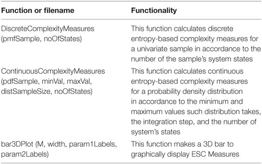
Table 1. Summary for discrete and continuous complexity Octave/Matlab functions.

In Appendix C, numeric results for the code examples are provided (three machine learning datasets² (Fanaee-T and Gama, 2013; Lichman, 2013) and two probability distributions). Furthermore, in Appendix D, we provide an example on the use of our complexity measures to analyze a system at different timescales.

2. Method: Emergence, Self-Organization, and Complexity

In this section, we describe the statistical measures of E, S, and C. Discrete measures were defined in a previous study presented in Fernández et al. (2014), latter extended for continuous probability distributions (Santamaría-Bonfil et al., 2016). This package is limited to the aforementioned measures. Proofs, advantages, and limitations are defined and discussed in Fernández et al. (2014) and Santamaría-Bonfil et al. (2016). Furthermore, for simplicity, differences between discrete and the continuous will be mentioned when necessary.

Many notions of Emergence describe it as novelty (between scales, in time, or within a process). E can be understood as new global patterns which are not present in the system’s components. More precisely, for a discrete probability distributions, E measures the average ratio of uncertainty a process produces by new information that is a consequence of changes in (a) dynamics or (b) scale. For continuous distributions, E interpretation is constrained to the average uncertainty a process produces under a specific set of the distribution parameters (e.g., the SD value for a Gaussian distribution) (Santamaría-Bonfil et al., 2016). Formally, the discrete and continuous E are defined as follows:

$E_D=-K{\displaystyle {\sum }_{i=1}^N{p}_i{\text{\hspace{0.17em}log}}_2{p}_i}$

$E_C=-K({\lim }_{\mathrm{\Delta }\to 0}H(X^{\mathrm{\Delta }})+{\log }_2(\mathrm{\Delta }))$ (1)

E_D in equation (1) corresponds to the discrete E, where p_i = P(X = x) is the probability of the element i. E_C in equation (1) corresponds to the continuous E. Note that the latter is rather a quantized version of the differential entropy, where X^Δ corresponds to discretized version of X, and Δ is the integration step. On the other hand, K is a normalizing constant that constrains E within the range 0 ≤ E ≤ 1. It is estimated as

$K=\frac{1}{{\log }_2(b)},$ (2)

where b corresponds to the system’s alphabet size: the number of bins of a probability mass function, or, in the continuous case, to the states that satisfies P(x_i) > 0. More importantly, the denominator of equation (2), log₂(b), corresponds to the maximum entropy for a distribution function with alphabet size of b. Consequently, E can be understood as the ratio between the entropy for given distribution H(X), and the maximum entropy for the same alphabet size H(U), $E=\frac{H(X)}{H(U)}$.

It is also worth noting that, E_D = 0 is only achievable when the entropy for a given probability distribution is such that H(X) = 0, which corresponds to the entropy of a Dirac delta distribution. However, in the continuous case the differential entropy of a Dirac delta or a discrete value is −∞. Nonetheless, differential entropy only becomes negative when the probability distribution becomes extremely concentrated in very few states. Thus, when calculating our statistical continuous complexity measures, we set H(x_i) = 0 iff H(x_i) < 0.

Self-organization, in its most general form, can be seen as a reduction of entropy (Gershenson and Heylighen, 2003). S is the complement of E, thus, self-organization is related to order and regularity due changes in the process dynamics or scale. In this sense, an entirely random process (e.g., uniform distribution) has the lowest organization and a completely deterministic system one (Dirac delta distribution) has the highest. S is defined as

$S=1-E=1-\left(\frac{H(P(X))}{H(U)}\right),$ (3)

such that 0 ≤ S ≤ 1.

Complexity comes from the Latin plexus, which means interwoven. Thus, something complex is difficult to separate. This means that its components are interdependent, i.e., their future is partly determined by their interactions. Complexity represents a balance between change and regularity (Kaufmann, 1993), which allows systems to adapt in a robust fashion. Regularity ensures that information survives, while change allows the exploration of new possibilities, essential for adaptability. In this sense, complexity can also be used to characterize living systems or artificial adaptive systems, especially when comparing their complexity with that of their environment (Fernández et al., 2014). More precisely, this function describes a system’s behavior in terms of the average uncertainty produced by emergent and regular global patterns as described by its probability distribution. Thus, the complexity measure is defined as

$C=4\cdot E\cdot S,$ (4)

such that, 0 ≤ C ≤ 1. C is only maximal when E and S are equal (i.e., E = S = 0.5). In Fernández et al. (2014) they showed that for a variable with only two states, the highest C is achieved when one of the states is highly probable, i.e., ≈0.89. Thus, it infers that a system which concentrates its dynamics into few highly probable states with many less frequent states, displays high complexity (e.g., a power-law distribution). C becomes 0 for equiprobable distributions.

3. Functions of Complexity Measures

The complexity of different phenomena can be calculated using entropy-based measures. However, to obtain meaningful results, users must first determine the adequate function to be employed for their problem (e.g., should a raw sample or an estimated probability distribution function be used?). In this section, we describe two functions for complexity: DiscreteComplexityMeasures, and ContinuousComplexityMeasures. We provide details on the inputs and outputs required by these complexity functions. In addition, we also provide a graphical function to display emergence, self-organization, and complexity (ESC); we take no authorship of it since it is freely available on the internet³; nonetheless, in the next section, we provide details of its functionality.

3.1. Functions Definition

DiscreteComplexityMeasures, and ContinuousComplexityMeasures are briefly summarized at Table 1. In the following, inputs and outputs are detailed.

3.1.1. Inputs

1. DiscreteComplexityMeasures(pmfSample, noOfStates)

(a) pmfSample is a vector of size n × 1 which corresponds to n real values displayed by a given system, e.g., a time series.

(b) noOfStates is an integer ≥2 that defines the number of states to coarse grain the given sample. If it is empty, a heuristic is used to calculate the number of system states.

2. ContinuousComplexityMeasures(pdfSample, varargin)

(a) pdfSample is a vector of size n × 1, which contains the n probability values assigned by the probability distribution function (i.e., f(x) = P(x)).

(b) Additional parameters are:

i. minVal, it’s a real value corresponding to the minimal value where the PDF will be evaluated.

ii. maxVal, it’s a real value corresponding to the maximal value where the PDF will be evaluated. It is strictly necessary that minVal < maxVal.

iii. distSampleSize, is an integer value which corresponds to an approximate sample size. This value is used to estimate the integration step $\mathrm{\Delta }=\frac{maxVal-minVal}{distSampleSize}$.

iv. noOfStates is an integer value used to define the number of possible states a system can take. As its discrete counterpart, it should satisfy that ≥2. In particular, noOfStates should be large to satisfy 0 ≤ E, S, C ≤ 1. If not provided, a heuristic is employed to obtain it.

3. bar3DPlot(M, width, param1Labels, varargin)

(a) M is n × 3 or n × m matrix. For the former, rows correspond to a feature of a system whereas its columns are the corresponding E, S, C, respectively. For the latter, columns are rather a parameter of the system, thus, only one ESC measure can be displayed at a time.

(b) width determines each bar size, this value ranges from

(c) 0 < width ≤ 1.

(d) param1Labels this parameter is n × 1 label matrix. It contains the corresponding labels for each row of M.

(e) When M is a n × m matrix, additional labels are required. param2Labels is n × 1 label matrix which contains the corresponding labels for each column of M.

3.1.2. Outputs

Complexity measure functions return 4 elements: three mandatory outputs Emergence, Self-organization, Complexity, and an optional one, which corresponds to data’s discrete or continuous entropy.

3.2. Results Interpretation

E, S, and C measures provide a big picture about the expected uncertainty that belongs to a system in terms of its probability distribution product of (a) a reduction/increase of system’s states (Gershenson and Fernández, 2012), or (b) the concentration/homogenization of the probability distribution (Santamaría-Bonfil et al., 2016). E is able to measure the change in scale given a process that transforms information (Gershenson and Fernández, 2012). For instance, E can be expressed as $E=\frac{H_{out}(x)}{H_{in}(x)}$, where H_in is the initial entropy for a system, and H_out = f(H_in) is H_in transformed by process f. On the other hand, for a given probability distribution either discrete or continuous, if E is close to 1, the system shows similar probability for most of its states. Otherwise, if E ≡ 1, all states are equiprobable. Thus, if 0 < E ≪ 1, then, system’s states distribution have few states with a considerable amount of the probability, whereas if 0 ≪ E < 1 then, the states of the system are more evenly distributed. Since S is the complement of E, the above mentioned descriptions apply in a conversely way to S. In this context, if S ≡ 1, the system can be considered to be predictable since a single state x_j has P(x_j) ≈ 1. This interpretation of E and S is shared by other Shannon-based measures like LMC Complexity and statistical diversity (Lopez-Ruiz et al., 1995; Jost, 2006) (e.g., the disequilibrium of a crystal = the diversity of a population with exactly 1 species = S_max = 1).

On the other hand, C = 1 only when E, S = 0.5. Such scenario is given when a single or few state are highly concentrated in terms of their probability, with many other states with lesser probabilities. In this regard, C becomes 0 when the distribution resembles a uniform distribution or a Dirac delta. Moreover, higher values of C are required in order to the probability distribution remains. It should be noted that a system with 5 states is considered as follows: one state has p(s₁) = 0.8 and the remaining 4 states have equal probability p(s_{2, …, 5}) = 0.05 hence C = 0.9988. This behaviour can be observed in the Gaussian distribution case discussed in Appendix C.

3.3. Issues and Limitations

Some of the known issues, considerations, and limitations of this package are as follows:

1. The statistical measures proposed are mainly based on Shannon’s discrete and differential entropy (i.e., H(X)) per symbol.

2. Our proposed measures only consider I.I.D. random variables. Thus, conditional time relations or strings size > 1 are not considered. The former is particularly important when analyzing a distribution. For instance, if a discrete sequence of repeating points, e.g., 0, 1, 2, 0, 1, 2, … is analyzed in terms of each number, the distribution will resemble a uniform distribution; hence, E = 1. However, if the states of the system are strings of 3 elements, the distribution will be Dirac delta S = 1.

3. In order to obtain some preliminary results when calculating continuous complexity, it should be considered the size of the integration step Δ. In this context, if Δ ≈ 0 then H(x) = −∞, which could induce a spurious decay of E_C values (interested reader please refer to Santamaría-Bonfil et al. (2016) for more details).

4. Emergence value is understood as E = K*H(X) constraining it to 0 ≤ E ≤ 1 by the normalizing constant K (Fernández et al., 2014). This constant value is calculated as K = 1/log(b) where b is the system’s alphabet size. Since, log(b), corresponds to the maximum entropy for any probability distribution with b symbols, E is the ratio between the entropy for a given distribution P(X), and the maximum entropy for the same alphabet size (Santamaría-Bonfil et al., 2016). Therefore, if b is not provided, a heuristic is employed with the aim to compute the total number of symbols from P(X) that satisfies p(x) > 0 (both for discrete and complexity measures).

5. These ESC measures are univariate.

4. Code Example: ExampleComplexityMeasures

In this section, we present an example that shows the functionality of our complexity measures (additional details are provided at Appendix C). First, we present the overall functionality of the example and how it should be edited. Octave 4.0.3. or Matlab 2013a are required to run these complexity functions. We highly recommend to the reader to use as templates the examples and complexity measures from the publicly available Entropy-based Complexity repository.

The example ExampleComplexityMeasures, is basically divided in two sections (1) discrete examples, and (2) continuous examples. In either case, ESC measures are simultaneously calculated, and stored in variable ESC to make a 3D Bar plot as follows:

[Emrgnc, SlfRgnztn, Cmplxty] = …

DiscreteComplexityMeasures(pmfSample, noOfStates);

ESC = [Emrgnc, SlfRgnztn, Cmplxty];

typeLabel = [’Feature1’;’Feature2’];

figure (1);

width = 1;

bar3DPlot(ESC,width,typelabes);

4.1. How to Modify the Example?

First, you must choose between discrete or continuous examples. Next, you need to specify the working directory and the dataset. Some datasets from the University of California Irvine were provided in advance (UCI) (Lichman, 2013) in mat format: (a) frequency of three types of solar flares per 24 h, (b) the bicycle rides made per day and hour for a station within a bicycle sharing system, and (c) household electric consumption per minute for a whole house metering and kitchen submetering. These must be downloaded to the working directory. For the example of continuous complexity measures, a probability distribution data are generated on the fly. Any other dataset to work with must be in mat format.

The working directory is specified (a) via Matlab/Octave user interface, or (b) by setting the path via code as is shown.

filePath = ’C:\HereSetYourPath\’;

Next, you must choose the type of complexity measure: 1 for discrete and 2 for differential.

complexityType = 1; %Discrete complexity measures

%complexityType = 2;%Continuous complexity measures

If discrete complexity function is chosen:

Specify the dataset to be employed:

dataSet = 1; load([filePath SolarFlaresData]);

% dataSet = 2; load([filePath BikeSharingData]);

% dataSet = 3; load([filePath

            HouseElecCnsmptData]);

Also, you may specify the number of states (noOfStates) the system will have, 10 is an educated guess.

noOfStates = 10;%Number of states of the system

Finally, calculate ESC measures as follows:

[Emrgnc,

SlfRgnztn,

Cmplxty] = DiscreteComplexityMeasures(…

            pmfSample,noOfStates);

For illustrative purposes, we chose as pmfSample the household electric consumption described in Appendix C. The corresponding results are shown in Figure 1.

FIGURE 1

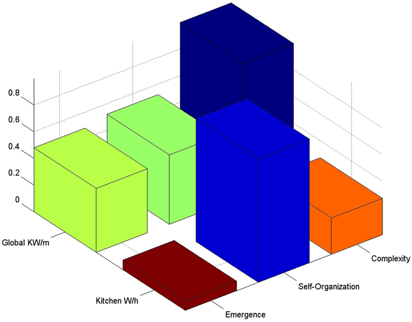
Figure 1. Discrete E, S, and C for a single household electric consumption. These data correspond to time series of energy consumption per minute for a whole house and its kitchen. Note that the electricity consumption for the whole house has complexity near 1, while the kitchen is rather highly self-organized. In the former, the results imply that a single or few energy consumption states concentrate most of the probability (i.e., regular patterns) with many new emergent states of usage. In the latter, kitchen’s energy consumption is more regular and more predictable. In fact most of the time kitchen will not consume electricity (91% of the probability is concentrated in the 0 energy consumption state). Kitchen also displays a C ≈ 0.27, which is the result of its periodic usage (e.g., meals during workweeks).

If continuous complexity function is chosen:

Probability Density Functions are used to estimate Gaussian and Power-Law (PL) distributions. In the former, a pre-programmed language function is employed, whereas in the latter, we implemented our own probability function. In either case, some parameters are required: distSampleSize and distParamNum. The first determines the integration sampling step. The second is the number of parameters that our probability distribution will have (in the Normal distribution case, different σ values are used, whereas, in the PL distribution, distinct x_min and α values are employed).

distSampleSize = 100000;

distParamNum = 10;

Next, specify variable pdfType to select either, 1 Gaussian, or 2 PL distribution.

pdfType = 1;% Gaussian Distribution

% pdfType = 2;% Power-law Distribution

Also, you must specify the noOfStates as in the discrete case. Variable plotPDFOn = {0, 1} can be used to plot PDF’s for the different parameters. Finally, calculate ESC measures for a PDF by calling the function as follows:

[Emrgnc,

SlfRgnztn,

Cmplxty] = ContinuousComplexityMeasures(

        pdfDist,minVal,maxVal, …

       distSampleSize,noOfStates);

For illustrative purposes we chose as the pdfSample a power-law with parameters x_min = 3 and α = 2, …, 11. The corresponding results are shown in Figure 2.

FIGURE 2

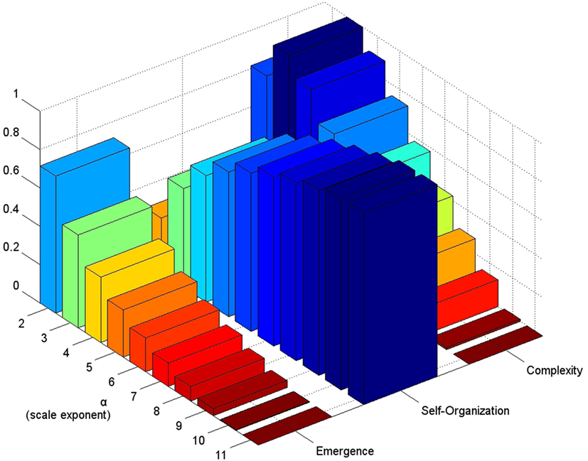
Figure 2. Continuous E, S, and C for a power-law with a fixed x_min = 3 and scale exponents α = 2, …, 11. Note that as the scale exponent grows, E decays product of the concentration of distribution around the x_min value. However, even for α = 11, a considerable amount of complexity is displayed C ≈ 0.37. The latter is product of the heavy-tail of the distribution. Also note that C is high for 2 ≤ α ≤ 4 where C ≈ 0.95, 0.99, 0.93, respectively. The max C can be shifted to lower or higher scale exponents by x_min, which may be convenient to describe real-world phenomena.

5. Discussion

In this paper, we presented two functions to calculate entropy-based complexity measures: Emergence, Self-Organization, and Complexity. These measures can be employed for discrete samples or continuous probability distributions. The inputs and outputs for these two functions were described, and a code example for testing complexity functions was provided. Additionally, code snippets and dataset descriptions are provided in Appendixes A, B, and C, respectively.

Additional notes need to be made. First, for pedagogical purposes these functions were developed using GNU Octave language. However, they can be easily extended to R or Python. Note that for a fast computation process, the implementation of these measures on other languages will require vector and matrix operations, loop usage is discouraged. Second, these functions only are designed to calculate discrete and continuous complexity of univariate systems. Thus, a measure for multivariate systems is required. A fast proxy for multivariate entropy calculation could be the summation of each feature entropy. Consequently, Emergence could be calculated as the ratio of $\frac{{\displaystyle {\sum }_i}H\left(X_i\right)}{N{\displaystyle {\sum }_i}lo{g}_2\left(b_i\right)}$, where N is the number of system variables, and b_i is the alphabet for each variable. However, further research about this issue is required. Third, a further extension of this research includes the usage of the continuous entropy to calculate discrete complexity measures to provide more sensible results for any given probability mass function. Also, because these measures only describe the complexity at the level of symbols in the alphabet rather than on strings, conditional entropy should be used in future work. Such function can provide the average entropy growth for both, IID random variables and stochastic processes. Particularly the latter feature would be convenient for analyzing the complexity of time series and dynamical processes with memory.

Author Contributions

GS-B designed and coded ESC discrete and continuous Matlab/Octave functions and performed the experiments. GS-B, CG, and NF conceived and designed the experiments and wrote the paper.

Conflict of Interest Statement

The authors declare that the research was conducted in the absence of any commercial or financial relationships that could be construed as a potential conflict of interest.

The reviewer HZ declared a past co-authorship with one of the authors (CG) to the handling Editor, who ensured that the process met the standards of a fair and objective review.

Acknowledgments

The authors would like to thank Carlos Piña Ph.D. for the help in editing and proofreading this manuscript. GS-B was supported by the Consejo Nacional de Ciencia y Tecnología under the Cátedra-Conacyt contract 969.

Supplementary Material

The Supplementary Material for this article can be found online at https://www.frontiersin.org/article/10.3389/frobt.2017.00010/full#supplementary-material.

Footnotes

1. ^https://doi.org/10.5281/zenodo.166566.
2. ^http://archive.ics.uci.edu/ml.
3. ^http://stackoverflow.com/questions/24180890/3d-histogram-with-gnuplot-or-octave, accessed 30/10/2016.

References

Bandt, C., and Pompe, B. (2002). Permutation entropy: a natural complexity measure for time series. Phys. Rev. Lett. 88, 174102. doi: 10.1103/PhysRevLett.88.174102

PubMed Abstract | CrossRef Full Text | Google Scholar

Bar-Yam, Y. (1997). Dynamics of Complex Systems. Studies in Nonlinearity. Boulder, CO, USA: Westview Press.

Google Scholar

Fanaee-T, H., and Gama, J. (2013). Event labeling combining ensemble detectors and background knowledge. Prog. Artif. Intel. 2, 1–15. doi:10.1007/s13748-013-0040-3

CrossRef Full Text | Google Scholar

Fernández, N., Maldonado, C., and Gershenson, C. (2014). “Information measures of complexity, emergence, self-organization, homeostasis, and autopoiesis,” in Guided Self-Organization: Inception, Volume 9 of Emergence, Complexity and Computation, ed. M. Prokopenko (Berlin, Heidelberg: Springer), 19–51.

Google Scholar

Gauvrit, N., Singmann, H., Soler-Toscano, F., and Zenil, H. (2016). Algorithmic complexity for psychology: a user-friendly implementation of the coding theorem method. Behav. Res. Methods 48, 314–329. doi:10.3758/s13428-015-0574-3

PubMed Abstract | CrossRef Full Text | Google Scholar

Gershenson, C., and Fernández, N. (2012). Complexity and information: measuring emergence, self-organization, and homeostasis at multiple scales. Complexity 18, 29–44. doi:10.1002/cplx.21424

CrossRef Full Text | Google Scholar

Gershenson, C., and Heylighen, F. (2003). “When can we call a system self-organizing?,” in Advances in Artificial Life, 7th European Conference, ECAL 2003 LNAI 2801, eds W. Banzhaf, T. Christaller, P. Dittrich, J. T. Kim, and J. Ziegler (Berlin: Springer), 606–614.

Google Scholar

Haken, H., and Portugali, J. (2017). Information and self-organization. Entropy 19, 18. doi:10.3390/e19010018

CrossRef Full Text | Google Scholar

Jost, L. (2006). Entropy and diversity. Oikos 113, 363–375. doi:10.1111/j.2006.0030-1299.14714.x

CrossRef Full Text | Google Scholar

Kaufmann, S. (1993). The Origins of Order. New York: Oxford University Press, Inc.

Google Scholar

Lichman, M. (2013). UCI Machine Learning Repository.

Google Scholar

Lizier, J. (2014). JIDT: an information-theoretic toolkit for studying the dynamics of complex systems. Front. Robot. AI 1:11. doi:10.3389/frobt.2014.00011

CrossRef Full Text | Google Scholar

Lopez-Ruiz, R., Mancini, H., and Calbet, X. (1995). A statistical measure of complexity. Phys. Lett. A 209, 321–326. doi:10.1016/0375-9601(95)00867-5

CrossRef Full Text | Google Scholar

Mitchell, M. (2009). Complexity: A Guided Tour. Oxford, UK: Oxford University Press.

Google Scholar

Prokopenko, M., Boschetti, F., and Ryan, A. (2009). An information-theoretic primer on complexity, self-organisation and emergence. Complexity 15, 11–28. doi:10.1002/cplx.20249

CrossRef Full Text | Google Scholar

Santamaría-Bonfil, G. (2016). GitHub Repository: Complexity Measures Functions.

Google Scholar

Santamaría-Bonfil, G., Fernández, N., and Gershenson, C. (2016). Measuring the complexity of continuous distributions. Entropy 18, 72. doi:10.3390/e18030072

CrossRef Full Text | Google Scholar

Soler-Toscano, F., Zenil, H., Delahaye, J., and Gauvrit, N. (2014). Calculating Kolmogorov complexity from the output frequency distributions of small Turing machines. PLoS ONE 9:e96223. doi:10.1371/journal.pone.0096223

PubMed Abstract | CrossRef Full Text | Google Scholar

Zenil, H., and Kiani, N. A. (2016). Low algorithmic complexity entropy-deceiving graphs. CoRR, 1–21. abs/1608.05972. arXiv:1608.05972.

Google Scholar

Zenil, H., Soler-Toscano, F., Kiani, N. A., Hernández-Orozco, S., and Rueda-Toicen, A. (2016). A decomposition method for global evaluation of shannon entropy and local estimations of algorithmic complexity. arXiv:1609.00110.

Google Scholar

Appendix

A. Discrete Complexity Measures

function [

emergence, …

selfOrganization, …

complexity, …

varargout] = …

DiscreteComplexityMeasures(stringSample, varargin)

%This function calculates Discrete Complexity Measures

%for discrete samples.

%First, we get the number of observations

%contained in the sample.

measLen = length(stringSample);

%If the number of states of the PMF

%is known beforehand

if(~isempty(varargin))

  %Calculate the marginal states probability

  no_States = varargin{1};

  margSttProb = (hist(…

    stringSample,no_States)./measLen)’;

else%Use an heuristic to obtain the PMF

  %Obtain the system’s unique states.

  sysStates = unique(stringSample);

  if(size(sysStates,2) > 1)

    sysStates = sysStates’;

  end

  %Get the length of the unique states.

  %And calculate the marginal states probability

  no_States = length(sysStates);

  margSttProb = zeros(length(sysStates), 1);

  for i = 1:no_States

    margSttProb(i,1) = (nnz(…

    ismember(…

    stringSample,sysStates(i))))/measLen;

  end

end

%Define the normalizing constant k

if(no_States = = 1)

  kConst = 1;

else

  kConst = 1/log2(no_States);

end

%Then, calculate entropy for all elements

%of the PMF with p(x) > 0

ind = margSttProb > 0;

entropy = Sum(margSttProb(ind,1).*log2(margSttProb(ind,1)));

%Calculate ESC measures

emergence = (-1)*kConst*entropy;

selfOrganization = 1 - emergence;

complexity = 4 * emergence * selfOrganization;

varargout1 = entropy;

end

B. Continuous Complexity Measures

function [

emergence, …

selfOrganization, …

complexity, …

varargout] = …

ContinuousComplexityMeasures(…

pdfSample, varargin)

minVal = varargin{1};

maxVal = varargin{2};

distSampleSize = varargin{3};

%Determine a integration interval Delta

%Remember that by definition

%for really small Deltas the entropy

%is negative and can become -infinity

Delta = (maxVal-minVal)/(distSampleSize);

%Use the provided Probability Distribution Function

%to determine the non-zero elements of the PDF

tempPdf = pdfSample;

ind = tempPdf > 0;

pdfNoZeros = sum(ind);

%Calculate Differential Entropy

%for the non-zero elements of the PDF

rightHandSide = -1*log2(Delta);

leftHandSide = (-1)*sum((Delta*tempPdf(ind)).*log2(tempPdf(ind)));

lmtEntrpy = rightHandSide + leftHandSide;

diffEntrop = lmtEntrpy + log2(Delta);

%K constant to be determined by 1) the number of

%no-zeros probability elements,

%2) a large value (i.e. the sample size)

if(if(length(varargin) < 4))

  if(distSampleSize < pdfNoZeros)

    kConst = 1/log2(pdfNoZeros);

  else

   kConst = 1/log2(distSampleSize);

  end

else

  kConst = 1/log2(varargin4);

end

modfDiffEntrop = diffEntrop.*kConst;

if(modfDiffEntrop < 0)

  emergence = 0;

  selfOrganization = 1;

  complexity = 0;

else

  emergence = modfDiffEntrop;

  selfOrganization = 1 - emergence;

  complexity = 4 *  (emergence  *  selfOrganization);

end

end

C. Experimental Description

In the following, experimental results are briefly described. To demonstrate the functionality of E, S, and C, two types of experiments were performed. On the one hand, discrete complexity measures using publicly available machine learning datasets were tested. On the other hand, continuous complexity measures using probability density functions were employed. For the discrete datasets, we used noOfStates = 10, whereas for the continuous case, we used noOfStates = 50. Only real-world datasets are described. For continuous complexity measures Gaussian and Power-Law distributions were used, however, since these probability distributions have been well documented elsewhere (Santamaría-Bonfil et al., 2016), no further details are provided. Results for the discrete measures for, the solar flares and the bike-sharing system datasets are shown in Figure 3, whereas for probability distributions are presented in Figure 4.

FIGURE 3

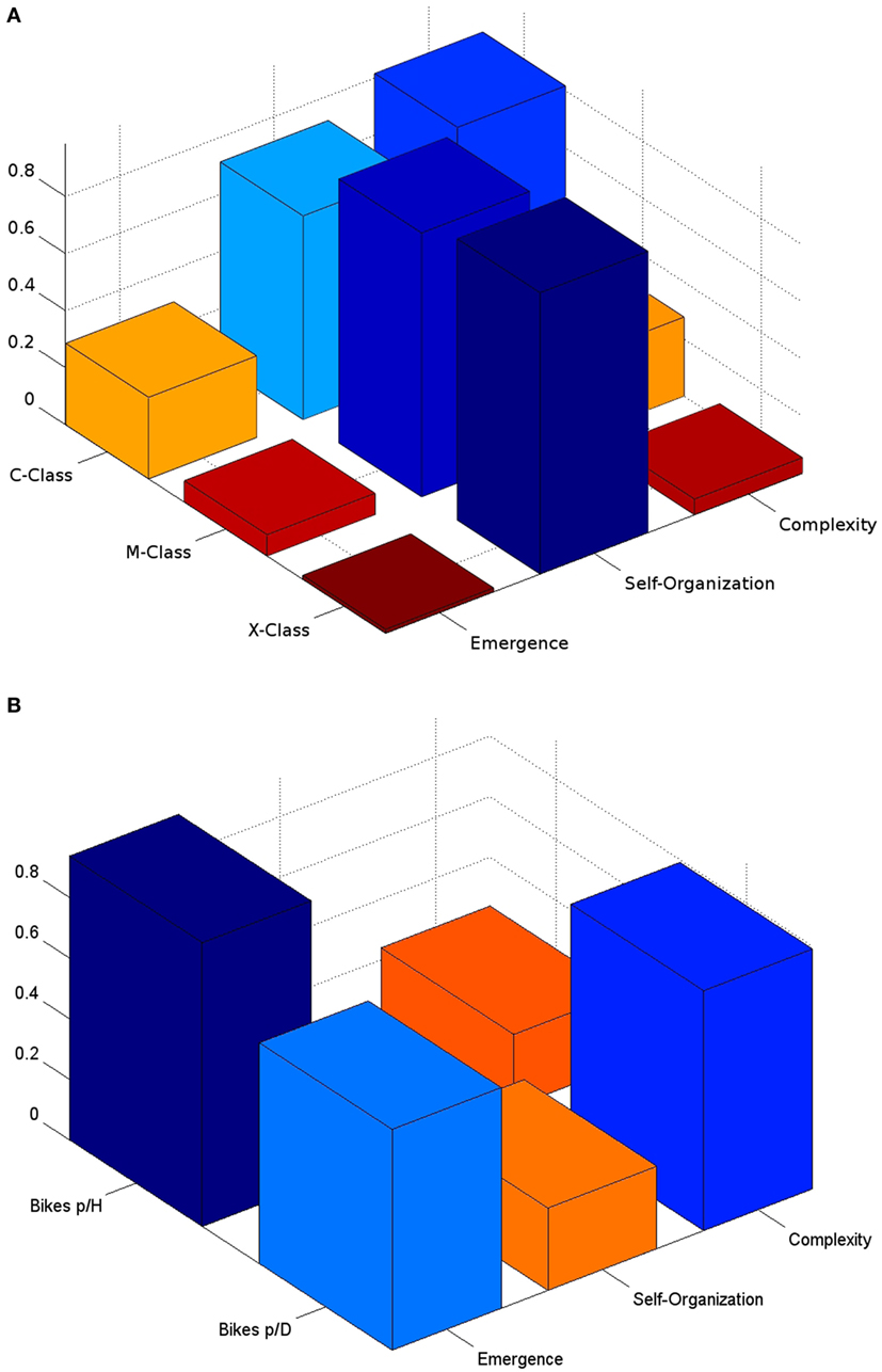
Figure 3. (A) Solar flares (B) bike-sharing system datasets. For the first set, high self-organization is appreciated for each type of solar flare class. As solar flares become larger in magnitude, its distribution becomes more organized (around a single state). Also, the number of possible states is reduced for larger magnitudes. Thus, the largest C is displayed by the common class. For the BSS dataset, we can observe that hourly usage is more uniformly distributed between its states, thus a higher E, than daily. Even while, hourly and daily usage have lower organization, the usage of the latter reaches a higher C ≈ 0.79, since its distribution is highly concentrated around the mean value, with many lower but uniformly distributed states around it.

FIGURE 4

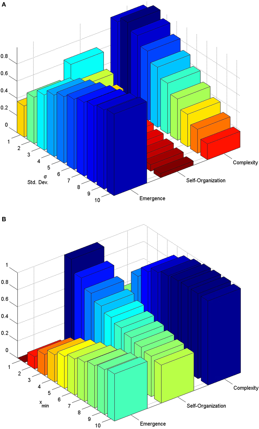
Figure 4. (A) Gaussian distribution (B) Power-law distribution. For the first, several SDs were tested σ = 1, …, 10. Note that the highest balance between S and E is constrained between 1 ≤ σ ≤ 3. As σ becomes larger, distribution becomes more uniform, thus, less complex. For the second, parameters were α = 5, and x_min = 1, …, 10. We can observe that as x_min value increases, so does the relation between a state with high probability and many others with lower one. It is known that for a system to be described as power-law its values must satisfy x_i > x_min. Thus, a high C may be a good proxy of the proper x_min value required (in this figure x_min ≥ 4).

C.1. Solar Flares

A solar flare occurs when magnetic energy that has built up in the solar atmosphere is suddenly released. UCI’s dataset contains three types of classes categorized by their magnitude and frequency. For each class, the number of solar flares of a certain class that occur in a 24-h period are counted.¹ The variables analyzed are three types of solar flares: (a) C-class flares, which are common, (b) M-class flares, which are flares of moderate size, and (c) X-class flares, which constitute flares of a severe magnitude.

C.2. Bike-Sharing System

Bike-sharing systems (BSS) are a new generation of urban mobility systems, composed by bicycles which are rented to subscribers for these to travel short to medium distances. These type of systems can be scrutinized from a large-scale statistic point of view.² In these experiments, BSS data consist in the total count of bicycle rentals per hour including both, casual and registered users. Further details can be obtained from Fanaee-T and Gama (2013), and UCI’s repository (Lichman, 2013).

C.3. Individual Household Electric Power Consumption Dataset

The need for a more efficient lifestyle requires to parametrize several aspects of human activities. Household electric consumption provides information not only to casual/conscious consumers but also to providers and grid managers. In these experiments, measurements of electric power consumption in one household with a 1-min sampling rate over a period of almost 4 years were used.³ We employed ~1 million observations of two variables: (a) the global household active power, which corresponds to global measures of the minute-averaged active power in kilowatts and (b) Kitchen energy sub-metering, which corresponds to measurements from a kitchen containing a dishwasher, an oven, and a microwave.

D. Example: Analyzing Timescales

In the previous section, numeric results of different phenomena and parameters of distributions were presented. In this section, we provide results for the analysis of multiple timescales. For such purposes, we employed the largest dataset available which is the household electric consumption. In the former example, only half of the dataset was employed. For this example, ~2 million points were used. The different timescales that were analyzed are minute, hour, day, week, and month. Further, we added another variable to the analysis, indoor comfort which consists of an electric water-heater and an air-conditioner. It was considered because indoor comfort represents around 60% of a building energy consumption.

First, we remove missing data points. Then, data were averaged in accordance to the aforementioned timescales. Next, we calculate Emergence, Self-organization, and Complexity, for the house’s global, kitchen, and indoor comfort active power. Results for the complexity measures are presented in Figure A1. The code for this example is provided in the Github repository (Santamaría-Bonfil, 2016) with the name Example2ComplexityMeasures.m.

FIGURE A1

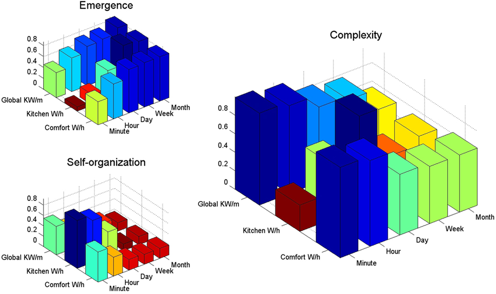
Figure A1. E, S, and C for the global, kitchen, and indoor comfort electric consumption for several timescales. For the global consumption, note that as the scale of the measures turns coarser, the probability distribution becomes more uniform. The highest Cs, few states with high probability and many emergent new states, is given for the minute/hour consumption. Moreover, even while the consumption of energy presents many new patterns for coarser measurement scales (i.e., week), cyclical and seasonal components remain considerable high (C ≈ 0.78). In fact, the same ESC behavior can be observed for the comfort energy usage give its high correlation with the whole house consumption. On the other hand, the kitchen electricity usage is highly self-organized (i.e., regular) for the minute and hour scales; however, self-organization quickly decays for the day time scale. Thus, kitchen’s daily electric consumption even while regular presents rich new patterns of usage (e.g., dinner with old friends).

Footnotes

1. ^https://archive.ics.uci.edu/ml/datasets/Solar+Flare.
2. ^https://archive.ics.uci.edu/ml/datasets/Bike+Sharing+Dataset.
3. ^https://archive.ics.uci.edu/ml/datasets/Individual+household+electric+power+consumption#.